Goals

Gain an awareness of Python libraries, their uses and potential.
Be able to install (where appropriate) and import libraries.
Practise using and writing code using these libraries.

Libraries

In Python, libraries are packages of pre-written code that usually contain functions and objects that can be imported into your own code. They are usually very efficient implementations of algorithms, models and procedures. In general if there is a library that does something you yourself would like to implement, it is better to use the library as it is probably well written, veified and tests, and efficient.

In this course you have already used some libraries, Ciw for simulating queueing systems, networkx for networks, numpy was used to reading in file (but is used for much more than this!), random for generating random numbers, and math for mathematical operations and constants.

There are two kinds of Python library:

Those in the standard Python library (e.g. math), these come pre-installed every distribution of Python. There is no need to install these libraries. Many are written by the same people who write Python itself.
Those not in the standard Python library (e.g. Ciw). In order to use these you will have to install them seperately uring pip.

Having said this, in this course we are using an Anaconda distribution of Python, which comes pre-installed with a number of popular libraries that are not in the standard Python library.

This tutorial is a demonstration of the uses of a number of libraries you may find useful during your studies. We will look at:

numpy for matrix and numerical operations,
matplotlib for creating plots,
pandas for data analysis,
scipy for statistical testing and other scientific procedures,
scikit-learn for machine learning.

Numpy

The power of this library is its efficiency in carrying out numeric computations, especially linear algebraic manipulation.

For example consider two matrices:

\[\mathbf{A} = \begin{pmatrix}3&4&-2\\2&1&-1\\7&-10&-5\end{pmatrix}\]

and

\[\mathbf{B} = \begin{pmatrix}1&5&4\end{pmatrix}\]

in numpy:

>>> import numpy as np

>>> A = np.array([[3, 4, -2], [2, 1, -1], [7, -10, -5]])
>>> A
array([[  3,   4,  -2],
       [  2,   1,  -1],
       [  7, -10,  -5]])

>>> B = np.array([[1, 5, 4]])
>>> B
array([[1, 5, 4]])

We can access the various elements of these matrices using indexing (like we have seen before with lists):

>>> A[0]
array([ 3,  4, -2])

>>> A[0][2]
-2

But also, a more efficent way to index is to use numpy indexing, like so:

>>> A[0, 1]
4

We can perform scalar multiplication:

>>> 5 * A
array([[ 15,  20, -10],
       [ 10,   5,  -5],
       [ 35, -50, -25]])

Raise to powers:

>>> np.linalg.matrix_power(A, 26)
array([[  15447237773911947,  278050279930415028,                   0],
       [   7723618886955973,  139025139965207515,                   0],
       [-262603042156503082,  525206084313006164,  154472377739119461]])

Perform matrix addition:

>>> A + A
array([[  6,   8,  -4],
       [  4,   2,  -2],
       [ 14, -20, -10]])

And multiplication:

>>> np.matmul(B, A)
array([[ 41, -31, -27]])

And further linear algebraic manipulation, such as determinants and inverses:

>>> np.linalg.det(A)
20.99999999999997

>>> np.linalg.inv(A)
array([[-0.71428571,  1.9047619 , -0.0952381 ],
       [ 0.14285714, -0.04761905, -0.04761905],
       [-1.28571429,  2.76190476, -0.23809524]])

>>> np.matmul(A, np.linalg.inv(A))
array([[ 1.00000000e+00,  0.00000000e+00, -5.55111512e-17],
       [-2.22044605e-16,  1.00000000e+00, -8.32667268e-17],
       [ 1.33226763e-15, -1.33226763e-15,  1.00000000e+00]])

Numpy is also useful in other contexts, for example to create arrays of equally spaced numbers:

>>> # 20 numbers between 4 and 10:
>>> np.linspace(4, 10, 20)
array([ 4.        ,  4.31578947,  4.63157895,  4.94736842,  5.26315789,
        5.57894737,  5.89473684,  6.21052632,  6.52631579,  6.84210526,
        7.15789474,  7.47368421,  7.78947368,  8.10526316,  8.42105263,
        8.73684211,  9.05263158,  9.36842105,  9.68421053, 10.        ])

>>> # Or an array of numbers starting from 0, with space 0.2, ending at 30:
>>> np.arange(0, 30, 0.2)
array([ 0. ,  0.2,  0.4,  0.6,  0.8,  1. ,  1.2,  1.4,  1.6,  1.8,  2. ,
        2.2,  2.4,  2.6,  2.8,  3. ,  3.2,  3.4,  3.6,  3.8,  4. ,  4.2,
        4.4,  4.6,  4.8,  5. ,  5.2,  5.4,  5.6,  5.8,  6. ,  6.2,  6.4,
        6.6,  6.8,  7. ,  7.2,  7.4,  7.6,  7.8,  8. ,  8.2,  8.4,  8.6,
        8.8,  9. ,  9.2,  9.4,  9.6,  9.8, 10. , 10.2, 10.4, 10.6, 10.8,
       11. , 11.2, 11.4, 11.6, 11.8, 12. , 12.2, 12.4, 12.6, 12.8, 13. ,
       13.2, 13.4, 13.6, 13.8, 14. , 14.2, 14.4, 14.6, 14.8, 15. , 15.2,
       15.4, 15.6, 15.8, 16. , 16.2, 16.4, 16.6, 16.8, 17. , 17.2, 17.4,
       17.6, 17.8, 18. , 18.2, 18.4, 18.6, 18.8, 19. , 19.2, 19.4, 19.6,
       19.8, 20. , 20.2, 20.4, 20.6, 20.8, 21. , 21.2, 21.4, 21.6, 21.8,
       22. , 22.2, 22.4, 22.6, 22.8, 23. , 23.2, 23.4, 23.6, 23.8, 24. ,
       24.2, 24.4, 24.6, 24.8, 25. , 25.2, 25.4, 25.6, 25.8, 26. , 26.2,
       26.4, 26.6, 26.8, 27. , 27.2, 27.4, 27.6, 27.8, 28. , 28.2, 28.4,
       28.6, 28.8, 29. , 29.2, 29.4, 29.6, 29.8])

Matplotlib

This is the most popular Python library for producing plots. It is flexible enough to be able to create nearly most plots you will require in most styles, and it also has a simpler interface, pyplot, for quick and easy plotting.

We’ll demonstrate through examples.

Before we begin, in order for plots to display in Jupyter, we need the follwing line of code (this is only needed in Jupyter):

>>> %matplotlib inline

Next we’ll import pyplot, and create a line plot:

>>> import matplotlib.pyplot as plt

>>> x_vals = [1, 2, 3.5, 7, 8, 8.5, 9]
>>> y_vals = [-1.2, -1.1, 4, 3.5, 5.7, 5.7, 6]

>>> plt.plot(x_vals, y_vals)
>>> plt.show()
<matplotlib.figure.Figure at 0x10f995c18>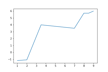

Using the same data, we can make a scatterplot (and let’s customise it a little):

>>> plt.scatter(x_vals, y_vals, c='red', s=150, marker='x')
>>> plt.show()
<matplotlib.figure.Figure at 0x10fbf3a90>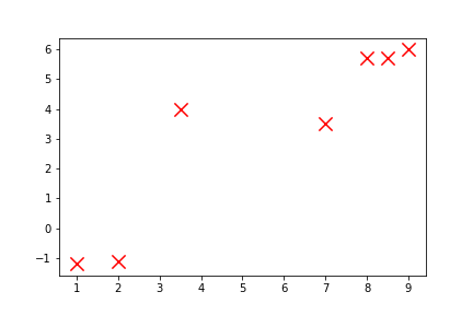

A vast number of other types of plot can be produced which can’t all be listed here. Below are examples of creating histograms and boxplots. First some random data is created (using the random library from the standard Python library):

>>> import random
>>> data = [random.lognormvariate(0.85, 0.45) for _ in range(350)]

>>> plt.hist(data)
>>> plt.show()
<matplotlib.figure.Figure at 0x10fd3a9e8>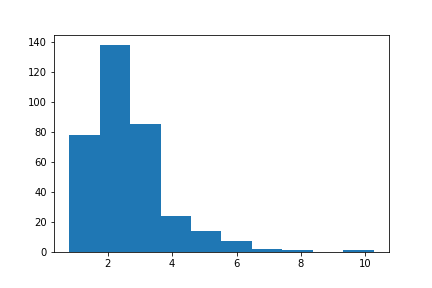

>>> plt.boxplot(data)
>>> plt.show()
<matplotlib.figure.Figure at 0x10ff78278>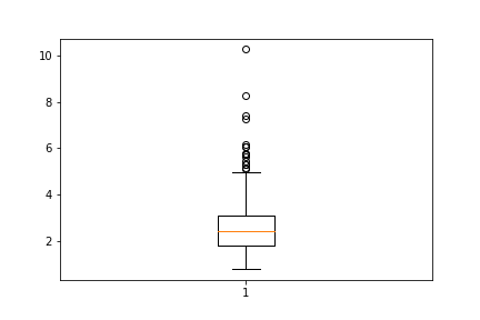

Finally matplotlib allows plots to be combined, customised and saved in a number of formats (experiment with .png, .svg and .pdf):

>>> plt.style.use('seaborn-whitegrid')
>>> plt.hist(data, alpha=0.7, color='darkorange', edgecolor='black', bins=[i*0.5 for i in range(21)])
>>> plt.ylabel('Frequency', fontsize=16)
>>> plt.xlabel('Values', fontsize=20)
>>> plt.title('My Histogram', fontsize=24)
>>> plt.xlim(0, 10)
>>> plt.savefig('histogram.pdf')
<matplotlib.figure.Figure at 0x110179da0>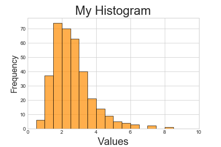

Pandas

Pandas is Python’s most popular library for data analysis and data manipulation. It is very useful for storing data in objects called ‘data frames’, which arrange data into useful and meaningful rows and columns. These data frames can be manipulated very efficiently for reshaping data, and performing data analyses on them.

To show an example, let’s read in a csv file (it can be downloaded from here if you’re following along), data of passengers on the Titanic:

>>> import pandas as pd
>>> data = pd.read_csv('titanic.csv')

And look at the first few rows:

>>> data.head()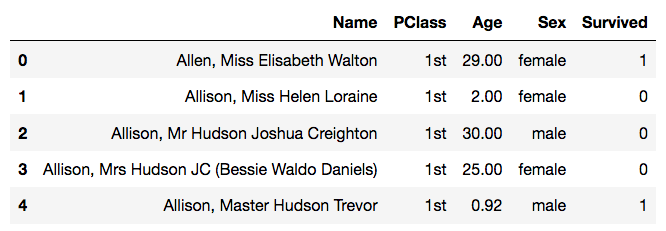

We can see that this data has 4 columns, the passengers’ name, their cabin class, their age and sex, and whether they survived or not.

We’ll use this to demonstrate some of pandas’ data manipulation methods.

>>> len(data) # number of observations (rows)
1313

>>> data.describe()  # Descriptive statistics for each numerical column of the data frame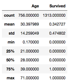

>>> data['Age'].head()  # just the 'Age' column (.head is used to get only the first 5 rows, to make the output easier to read)
0    29.00
1     2.00
2    30.00
3    25.00
4     0.92
Name: Age, dtype: float64

>>> data['PClass'].value_counts()  # Couting the number of each value in the 'PClass' column
3rd    711
1st    322
2nd    279
*        1
Name: PClass, dtype: int64

>>> data.groupby('PClass')['Age'].mean()  # The mean value of the 'Age' column for each unique value in the 'PClass' column
PClass
*            NaN
1st    39.667788
2nd    28.300142
3rd    25.208585
Name: Age, dtype: float64

>>> data[data['Age'] > 65]  # Filtering only those rows whose 'Age' value is greater than 65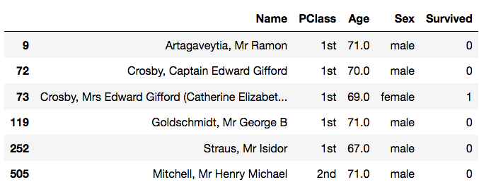

As you have seen above some of these methods can be combined, and pandas is very efficient at doing this. Sometimes simply reshaping data can give valuable insights, for example:

>>> data.groupby('PClass')['Survived'].mean()
PClass
*      0.000000
1st    0.599379
2nd    0.426523
3rd    0.194093
Name: Survived, dtype: float64

This gives the mean value of the ‘Survived’ column for each cabin class, that is for each value in the ‘PClass’ column. Knowing that ‘Survived’ is binary, its mean value is the proportion of passengers who survived.

Therefore by combining groupby and mean methods on the relevant columns, we can instantly see that there is a relationship between proportion of survivors and cabin class, with the lower cabin classes having a lower proportion of survivors.

Scipy

This scipy library is very versatile and has a number of functions and methods for conducting scientific procedures and algorithms. It is vast and has a number of specialised sublibraries. We’ll look at two of those here:

scipy.stats has a number of statistical functions for performing statistical tests and using probability distributions.
scipy.optimize has a number of algorithms for optimizing functions and curve-fitting.

Let’s use the Titanic data from above and consider it as a sample (it isn’t, it’s a population, but let’s consider it as a sample for the sake of demonstrating hypothesis testing). Let’s see if the average age of female passengers was equal to the average age of male passengers; using a independent sample t-test at the 1% level:

>>> import scipy.stats
>>> female_ages = data[data['Sex']=='female']['Age'].dropna()
>>> male_ages = data[data['Sex']=='male']['Age'].dropna()
>>> scipy.stats.ttest_ind(female_ages, male_ages)
Ttest_indResult(statistic=-1.5163397551570046, pvalue=0.1298525779150549)

A t-test was performed:

\(H_0\): The mean age of female passengers is equal to the mean age of male passengers.
\(H_1\): The mean age of female passengers is not equal to the mean age of male passengers.

We obtained a p-value of \(0.12385\dots\), and so at the 1% level the null hypothesis cannot be rejected, and there is not enough evidence to say that the mean ages of the genders differ.

Scipy also allows non-parametric tests if the observed data is not Normally distributed:

>>> scipy.stats.mannwhitneyu(female_ages, male_ages)
MannwhitneyuResult(statistic=62103.0, pvalue=0.03481292185615682)

A Mann-Whitney U test was performed:

\(H_0\): The median age of female passengers is equal to the mean age of male passengers.
\(H_1\): The median age of female passengers is not equal to the mean age of male passengers.

We obtained a p-value of \(0.0348\dots\), and so the 1% level null hypothesis cannot be rejected, and there is not enough evidence to say that the median ages of the genders differ.

Now using scipy.optimize, let’s see how we can minimise some function arbitrary function:

\[f(x, y) = \frac{1}{3} (x + 1)^2 + (y - 3)^2 - |xy|\]

First define this function as a Python function:

>>> def f(args):
...     x, y = args
...     return (1 / 3) * ((x + 1) ** 2) + ((y - 3) ** 2) - abs(x * y)

>>> f([5, 6]), f([8, 8]), f([-4, -3])
(-9.0, -12.0, 27.0)

>>> import scipy.optimize
>>> scipy.optimize.minimize(f, [0, 0])  # Give it x=0, y=0 as initial guesses
      fun: -39.999999999981355
 hess_inv: array([[ 5.9835314 , -3.00659123],
       [-3.00659123,  2.00053695]])
      jac: array([ 0.00000000e+00, -7.62939453e-06])
  message: 'Optimization terminated successfully.'
     nfev: 40
      nit: 9
     njev: 10
   status: 0
  success: True
        x: array([-21.999987  ,  13.99999137])

and this gives us the optimal values of \(x = -22\) and \(y = 14\).

Scikit-learn

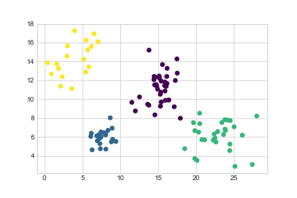
The final library we will look at is scikit-learn. This is Python’s machine learning library. It can implement a wide number of machine learning algorithms, but here we’ll just demonstrate a clustering algorithm.

First import a data set to demonstrate on (which can be downloaded here):

>>> data = pd.read_csv('plants.csv')
>>> data.head()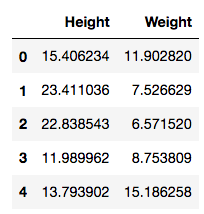

This has observations of plants with their height and weight recorded. A plot will show more information:

>>> plt.scatter(data['Height'], data['Weight'])
>>> plt.show()
<matplotlib.figure.Figure at 0x111f50710>

>>> plt.scatter(data['Height'], data['Weight'])
>>> plt.savefig('../../assets/plants-unclustered.png')
<matplotlib.figure.Figure at 0x1101e1d30>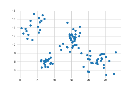

We can see there are four natural groupings. We’ll use k-means clustering to categorise these:

>>> import sklearn.cluster
>>> kmeans = sklearn.cluster.KMeans(n_clusters=4).fit(data)
>>> data['Cluster'] = kmeans.predict(data)

>>> data.head()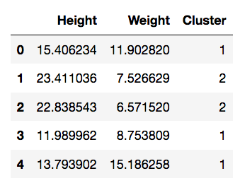

>>> plt.scatter(data['Height'], data['Weight'], c=data['Cluster'], cmap='viridis')
>>> plt.show()
<matplotlib.figure.Figure at 0x11aa68208>

Previous - Home - Next