The effect of variability on waiting times
This week I attended the CHOIR Healthcare Operations Research Summer School at the University of Twente in Enschede, the Netherlands. This was a fantastic opportunity where we learned about various operational research techniques that are currently being used in research and practice to solve healthcare problems (there were sessions on simulation, MDPs, inverse optimisation, and more). We discussed how to better engage with healthcare professionals to maximise impact, and most importantly meet some wonderful PhD students and researchers from all over the world.
One lively discussion session led by Prof. Erwin Hans saw us discussing how best to make an impact with our work. He outlined the successes of the CHOIR group, and the importance of understanding the differences in languages spoken by healthcare professionals and operational researchers. One important aspect of this is that health professionals like to speak of “optimising” something, whereas operational researchers tend to think about “reducing variability”, and that the latter tends to have more of an effect on systems. This is obviously evident in queueing systems, and this post aims to demonstrate that.
Deterministic vs. Markovian queues
The following is an example I like to give when explaining to friends what I study: Consider a single server queue. Customers arrive at the queue every 10 minutes, and service takes 10 minutes. We would not expect any queue to form, as customers follow a “one in - one out” pattern.
This is only true in the deterministic case, where customers arrive exactly 10 minutes apart, and customers spend exactly 10 minutes in service.
Now let’s consider the simplest mathematical model of a random queue. There is one sever. Customers arrive randomly, on average 10 minutes apart. Customers spend a random amount of time in service, on average lasting 10 minutes. Here when I say “randomly”, I mean that the distribution follows an exponential distribution. Mathematicians call this an \(M/M/1\) system, (Markovian arrivals and services) and have derived expressions for the expected waiting time of this system:
\[\mathbb{E}\left[W_q\right] = \frac{\rho}{\mu\left(1-\rho\right)}\] \[\rho = \frac{\lambda}{\mu}\]Where \(\lambda\) is the arrival rate and \(\mu\) is the service rate. In our system \(\lambda = 0.1\) (an arrival every 10 minutes) and \(\mu = 0.1\) (services last 10 minutes). It can quickly be seen that the traffic intensity \(\rho = 1\), and the expression for the average waiting time \(\mathbb{E}\left[W_q\right]\) approaches infinity.
The addition of variability in this system makes customers wait for an infinite amount of time!
General effect of variance
I’ll now use Python and the queueing simulation library Ciw to demonstrate how reducing the variability of a system may be sufficient to reduce waiting times. Here’s another similar blog post about this by Vincent Knight. Again consider a single server queue.
I’ll replace the distribution of service times with a Gamma distribution, in order to be able to increase the variance of service times without increasing the mean service time. Gamma distributions take two parameters \(\alpha\) and \(\beta\), and it’s mean and variance is given by the following expressions:
\[\mu = \alpha \beta\] \[\sigma^2 = \alpha \beta^2\]These can be rearranged to give:
\[\alpha = \frac{\mu^2}{\sigma^2}\] \[\beta = \frac{\sigma^2}{\mu}\]Choosing an arrival rate of 0.25, and a mean service rate of 2, I’ll simulate the system with increasing variances, for 100 time units. Note that I’m using trials, warm-up and cool-down times to follow best simulation practice. The code is given below:
>>> import ciw
>>> import numpy as np
>>> assert ciw.__version__ == '1.1.2'

>>> means = [1 for _ in range(1, 21)]
>>> variances = [0.25 * i for i in range(1, 21)]

>>> average_waits = []
>>> for v, m in zip(variances, means):
...     a = (m ** 2) / v
...     b = v / m
...     N = ciw.create_network(
...         Arrival_distributions=[['Exponential', 0.25]],
...         Service_distributions=[['Gamma', a, b]],
...         Number_of_servers=[1]
...     )
...     average_waits.append([])
...     for trial in range(50):
...         ciw.seed(trial)
...         Q = ciw.Simulation(N)
...         Q.simulate_until_max_time(140)
...         recs = Q.get_all_records()
...         waits = [r.waiting_time for r in recs if r.arrival_date > 20 if r.arrival_date < 120]
...         average_waits[-1].append(np.mean(waits))
Using seaborn I can plot the mean waiting time
for each value of \(\sigma^2\).
Seaborn’s tsplot method also gives the 95% confidence intervals.
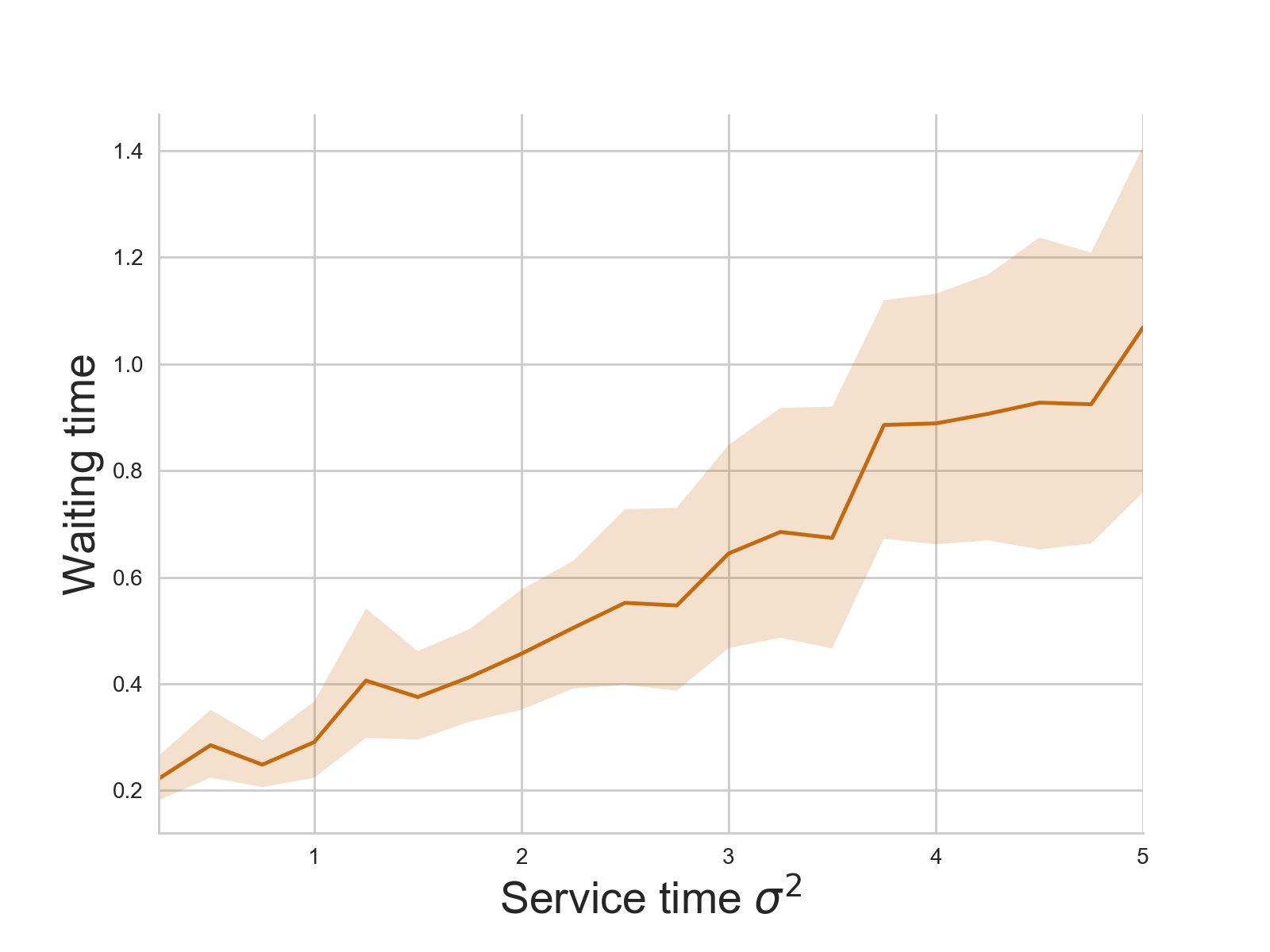
Increasing the variance of the service time, whilst keeping the mean fixed, increases the waiting time. In fact, with the parameters chosen, a fivefold increase in variance results in roughly a fourfold increase in the waiting time. (Note that using the Gamma distribution in this way, skewness, kurtosis, and other characteristics of the distribution may also change). This increase in variance also increases the variability of the waiting times.
Another experiment shows similar effects when increasing the variance of the arrivals:
>>> means = [2 for _ in range(1, 21)]
>>> variances = [0.25*i for i in range(1, 21)]

>>> average_waits = []
>>> for v, m in zip(variances, means):
...     a = (m ** 2) / v
...     b = v / m
...     N = ciw.create_network(
...         Arrival_distributions=[['Gamma', a, b]],
...         Service_distributions=[['Exponential', 2]],
...         Number_of_servers=[1]
...     )
...     average_waits.append([])
...     for trial in range(50):
...         ciw.seed(trial)
...         Q = ciw.Simulation(N)
...         Q.simulate_until_max_time(140)
...         recs = Q.get_all_records()
...         waits = [r.waiting_time for r in recs if r.arrival_date > 20 if r.arrival_date < 120]
...         average_waits[-1].append(np.mean(waits))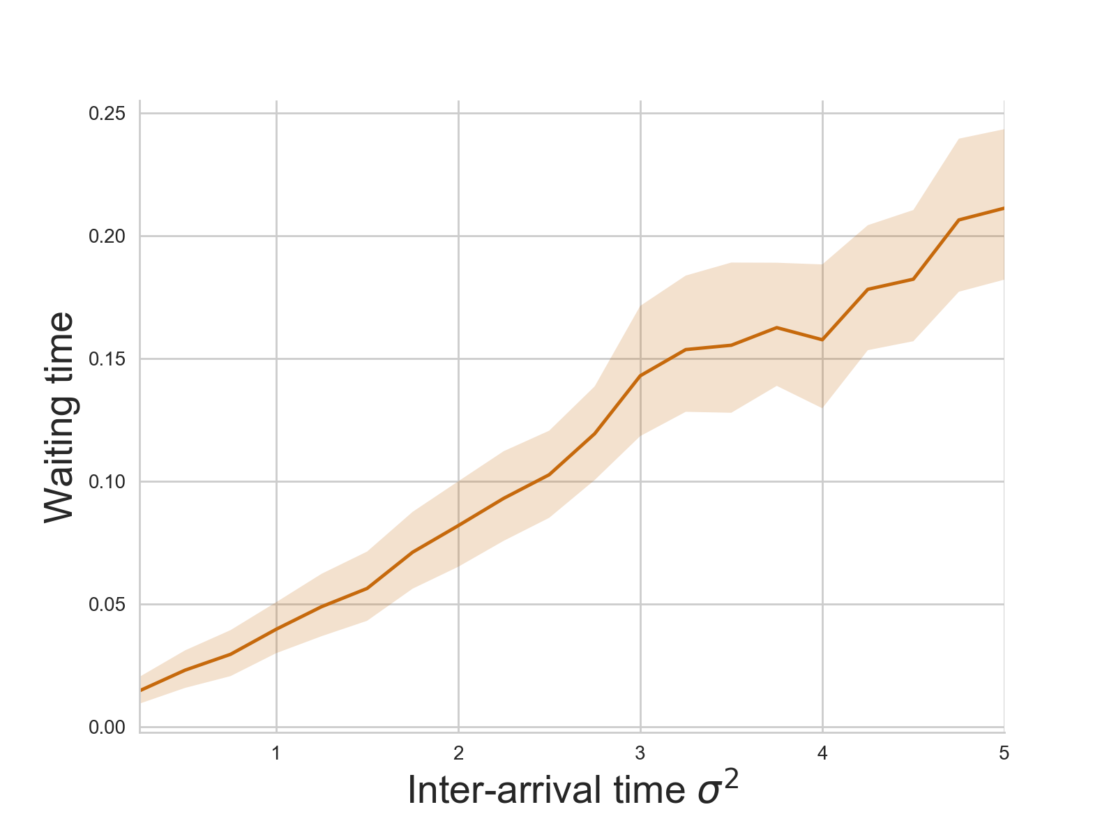
Again, increasing variance increases the waiting time.
These effects are evident in Kingman’s formula for the approximate waiting time of a \(G/G/1\) queue (general arrival and service distributions):
\[\mathbb{E}\left[W_q^{G/G/1}\right] \approx \mathbb{E}\left[W_q^{M/M/1}\right] \left(\frac{c_a^2 + c_s^2}{2}\right)\]where \(c_a^2\) is the coefficient of variation of the inter-arrival times, and \(c_s^2\) is the coefficient of variation of the service times. That is the variance divided by the mean squared. So as the variance of the arrivals and services increase, the corresponding coefficient of variation increases, and so the waiting time increases.
The toy systems discussed here are small, and are used to illustrate the importance of considering variability, especially in complex healthcare systems where variability arises often: emergency patients, staff sickness, surgery no shows, etc. This highlights the dangers of relying on means alone.