Creating maps with Geopandas
The last few week I began playing with creating maps in Python using the Geopandas library. It’s an amazing tool and I’ve become a big fan. The syntax is very similar to Pandas, and it works brilliantly with matplotlib too. To be honest the jump from using Pandas to Geopandas is tiny, and if you are comfortable with Pandas, there isn’t much work at all to understand Geopandas.
As part of my PhD work I looked into deprivation level in the five counties served by Aneurin Bevan University Health Board. I had a lot of help understanding LSOAs, polygons, and WIMD scores from my brother Rob who had produced these types of maps before in R. In this post I’ll show examples of plots I’ve created, and the simple code used to produce them.
Downloading Data
In my work I concentrated on five counties in south east Wales: Blaenau Gwent, Caerphilly, Monmouthshire, Newport, and Torfaen. I also needed to look at smaller more detailed areas. The smallest category of area in Wales are LSOAa (Local Super Output Areas), which are areas were between 1000 and 1500 people reside. Each LSOA has a code and a name: for example the LSOA containing Chepstow Castle is “St Mary’s”, and its code is W01001587.
In order to map LSOAs we need to know the shape and position of each area. These are defined by polygons. You can download these is geojson format from the ONS. Here’s the link that I used, which contains all LSOAs in Wales and England:
(Note that this dataset is huge: 34,753 LSOAs, each containing every vertex of the polygon that defines it. This will take a long while to download, ad will take some time to open with Geopandas. The first thing I did was filter and save another geojson file containing only the LSOAs of the five counties of interest.)
In addition to the polygons, I used two other data sets, containing information on WIMD deprivation measures for each LSOA (Welsh Index of Multiple Deprivation, a ranking where 1 denotes the most deprived LSOA, and 1909 denotes the most deprived LSOA), and the population over 60 years of age of each LSOA. I downloaded these from StatsWales and the ONS:
Reading Geojson
It’s easy to read in geojson to geopandas:
import geopandas as gpd
assert geopandas.__version__ == '0.3.0'

world = gpd.read_file('abuhb_world.geojson')
world is a GeoFataFrame object, which behaves exactly like a pandas
DataFrame.
After using Pandas to read in the deprivation and population datasets, I
combined the three data frames (using Pandas) such that world contains three
extra columns: WIMD, Over 60 a County:
>>> world
    objectid  lsoa11cd    lsoa11nm              lsoa11nmw   st_areasha  st_lengths      geometry                                                         WIMD  Over 60  County
0   34131     W01001325   Caerphilly 003A       Caerffili   003A        1.975810e+06    9595.912399  POLYGON ((-3.222590332332996 51.69544541936416...   219   342      Caerphilly
1   34132     W01001326   Caerphilly 003B       Caerffili   003B        1.418504e+06    7206.074574  POLYGON ((-3.218658752736475 51.69265017758838...   190   497      Caerphilly
2   34133     W01001327   Caerphilly 014A       Caerffili   014A        1.368584e+07    26141.148134 POLYGON ((-3.133625203219097 51.65362006379572...   1114  451      Caerphilly
3   34134     W01001328   Caerphilly 014B       Caerffili   014B        2.343212e+06    10639.884639 POLYGON ((-3.126845962218699 51.66067765558952...   815   370      Caerphilly
4   34135     W01001329   Caerphilly 014C       Caerffili   014C        4.799436e+05    4207.033238  POLYGON ((-3.124476654827622 51.63506150073896...   692   365      Caerphilly
Plotting a Map
Plotting a map of the polygons is easy:
world.plot()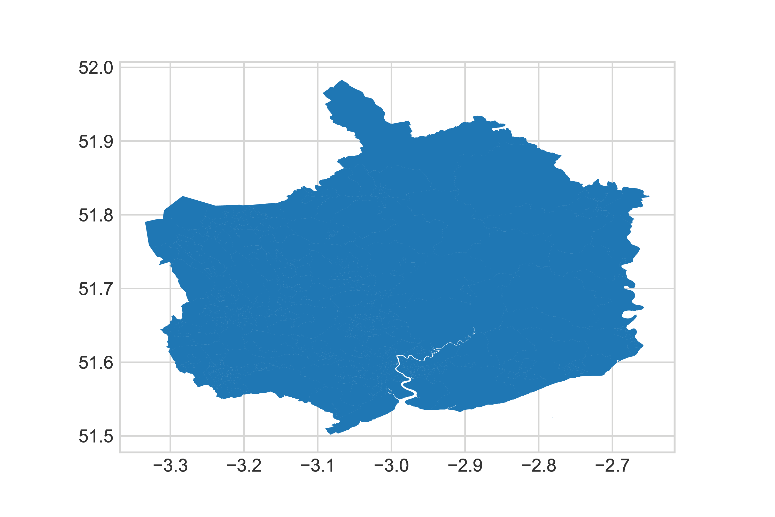
To designate how the polygons should be coloured, use arguments:
- Designate which column to use as values with
column - Designate the colormap to use with
cmap
You can also integrate with matplotlib’s object-orientated framework:
fig, ax = plt.subplots(1)
world.plot(column='Over 60', cmap='viridis_r', ax=ax)
ax.axis('off')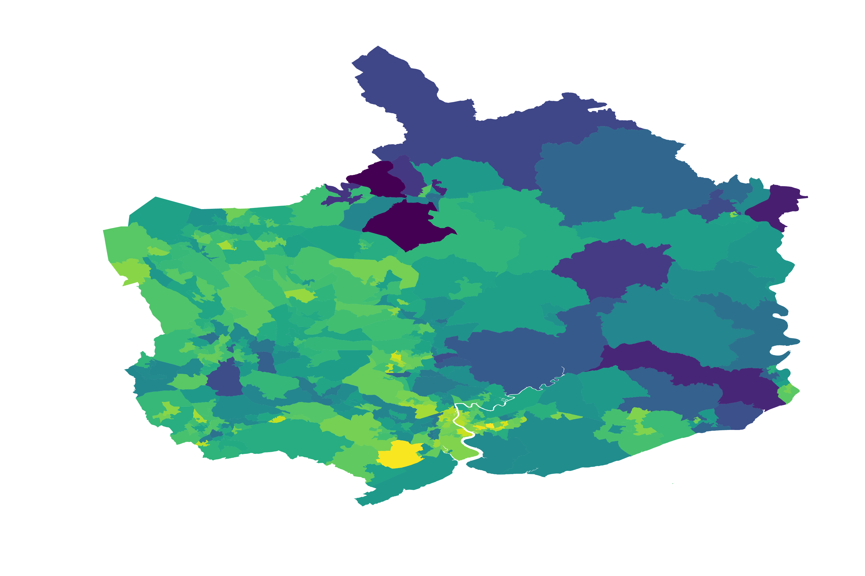
Manipulating Geometry
There are a number of methods for manipulating the geometry of the polygons.
Geopandas’ method of grouping is dissolve, which groups polygons with similar
properties and creates one big polygon from them.
Grouping LSOAs by county:
>>> counties = world.dissolve(by='County')
>>> counties
                geometry
Sir
Blaenau Gwent   POLYGON ((-3.219457536348314 51.74573457863166...
Caerphilly      POLYGON ((-3.123546981902226 51.58721244839312...
Monmouthshire   (POLYGON ((-2.781429130096552 51.5252840700888...
Newport         (POLYGON ((-2.903851574580124 51.6274883996199...
Torfaen         POLYGON ((-2.976496118298735 51.64839999700513...
We can find the centre point of a polygon with centroid:
counties['centroid'] = counties['geometry'].centroidOne use of finding a centre point of a polygon is to label polygons:
fig, ax = plt.subplots(1)
counties.plot(color='azure', edgecolor='black', ax=ax)
props = dict(boxstyle='round', facecolor='linen', alpha=1)
for point in counties.iterrows():
    ax.text(point[1]['centroid'].x,
            point[1]['centroid'].y,
            point[0],
            horizontalalignment='center',
            fontsize=10,
            bbox=props)
ax.axis('off')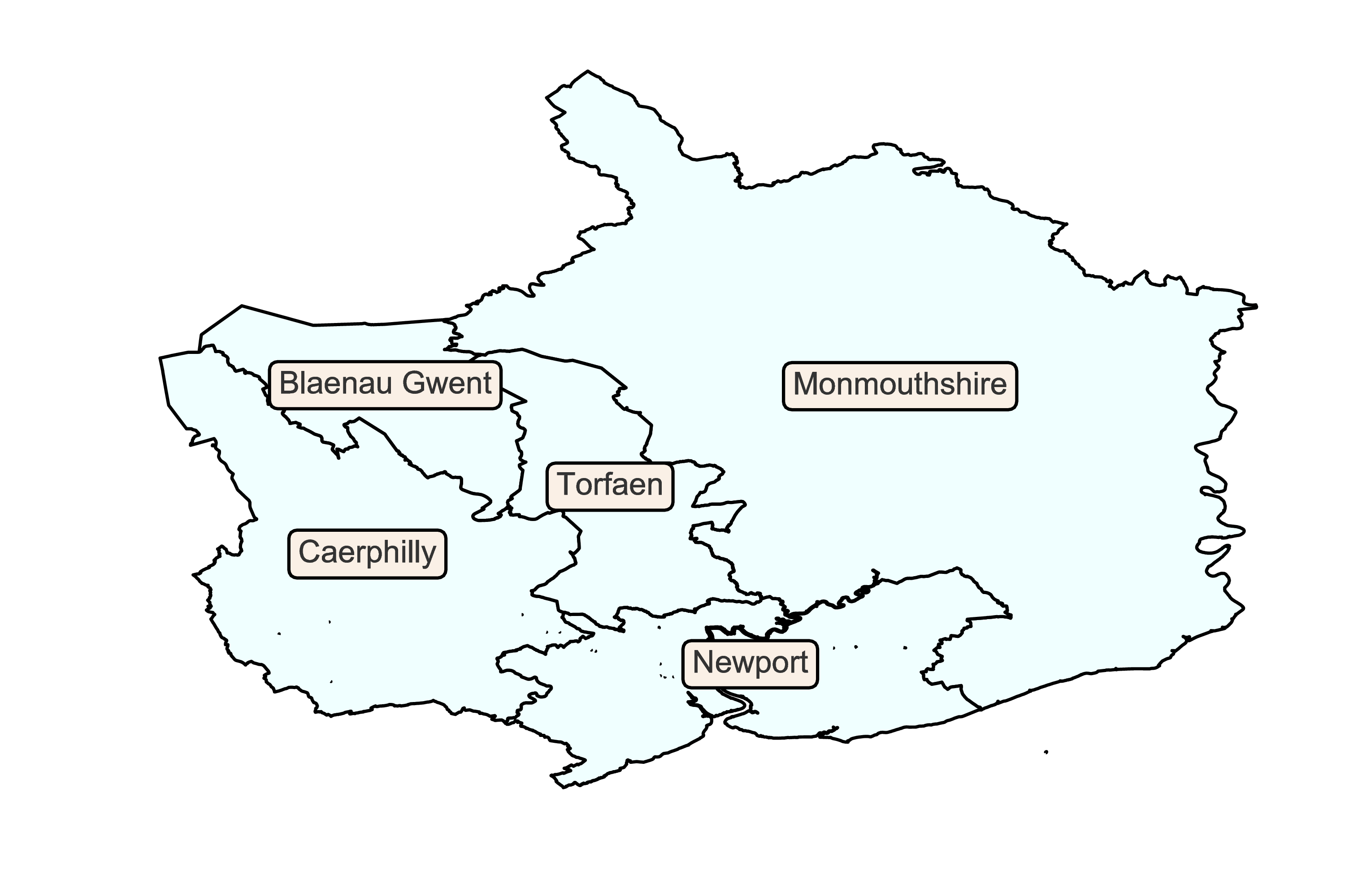
Geopandas also has a number of clever methods for dealing with different map projections
Conclusion
I have enjoyed playing with Geopandas, and a believe that the maps created are very beautiful.
Lastly, I will join two maps, LSOAs and counties, to look at deprivation.
Here I will use the GeoDataFrame counties to add black lines separating the
five counties.
fig, ax = plt.subplots(1, figsize=(10, 6))
world.plot(column='WIMD', ax=ax, cmap='viridis_r')
counties.plot(color='None', edgecolor='black', linewidth=2, ax=ax)
ax.axis('off')
vmin = world['WIMD'].min()
vmax = world['WIMD'].max()

# Create colorbar
sm = plt.cm.ScalarMappable(cmap='viridis_r', norm=plt.Normalize(vmin=vmin, vmax=vmax))
sm._A = []
cbar = fig.colorbar(sm)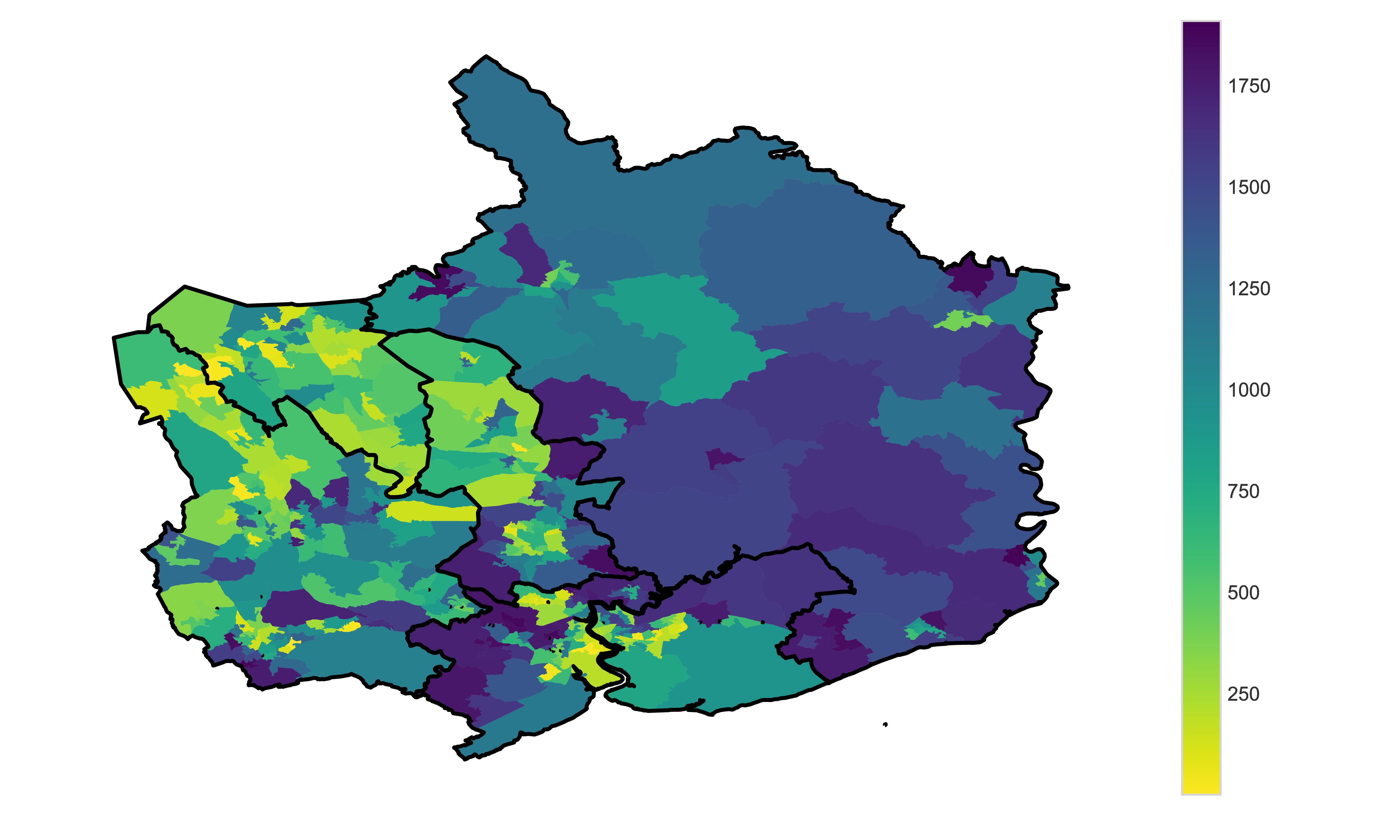
We can see that Monmouthshire has higher deprivation ranks than the other counties. Comparing with the map of population over 60 years of age, we can see that Monmouthshire has more older people than the other counties. In fact, the deprivation pattern and the pattern of population over 60 are awfully similar. Have we discovered something interesting? Are people over 60 more likely to move to areas with less deprivation?
Although the maps look nice, it’s difficult so say with these sort of maps, because geographic information has so many covariates. In this case, WIMD scores are calculated from a number of covariates. One of them is unemployment: retired people do not count as unemployed, so the more older people there are in an area, unemployment will fall. It seems that a number of WIMD’s covariates are affected by older people, therefore we cannot draw any conclusions here.
Despite this, Geopandas is a fantastic tool, it produces very pretty maps, and is easy to use if you are already familiar with Pandas.