Deadlock in Queueing Networks
I recently had my first journal paper accepted, written with my PhD supervisors Prof. Paul Harper and Dr. Vincent Knight. The paper is titled “Modelling Deadlock in Open Restricted Queueing Networks”, published in the European Journal of Operational Research.
In this paper we explore an under-investigated phenomenon of queueing networks: deadlock. First we look at discrete event simulation, and present a method of detecting when deadlock occurs. Then, taking advantage of this method, and by building analytical models of deadlocking queueing networks, we investigate what affects the time until deadlock is reached.
What is deadlock?
The image of gridlock below is a great analogy to deadlock: the red cars are blocked from continuing their journey by the blue cars, who are blocked by the yellow cars, who are blocked by the green cars, who are blocked by the red cars. The red cars are blocking themselves!
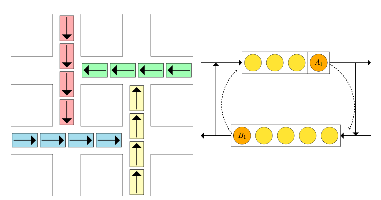
An underpinning concept of restricted queueing networks is blocking. This is where customers, after finishing service are trying to join another node, but cannot as the queue is full. Now they must remain with their server (who cannot serve any other customer in the meantime) until space becomes available at their intended destination.
These blocking rules give rise to a situation (illustrated above) where two or more customers may be blocking one another, and waiting for the other to move before they themselves can move. They are blocking themselves.
This situation grinds the system to a halt.
Detecting deadlock
Allowing simulations to reach deadlock is problematic. Without the ability to detect when deadlock occurs in discrete event simulations, a large chunk of the simulation time may have no events, thus skewing performance measures. Without the ability to detect deadlock in discrete event simulations, mechanics cannot be put into place to resolve the deadlocks as would happen in reality.
We present a graph theoretic result that indicates when deadlock occurs, by defining a state digraph \(D(t) = (V, E(t))\):
- The set of vertices \(V\) corresponds to the set of servers of the queueing network.
- The set of edges \(E(t)\) corresponds to the set of all blockage relations: If a customer at the \(k^{\text{th}}\) server of node \(i\) is blocked from entering node \(j\), then there are directed edges from the vertex corresponding to node \(i\)’s \(k^{\text{th}}\) server to every vertex corresponding to the servers of node \(j\).
For example:
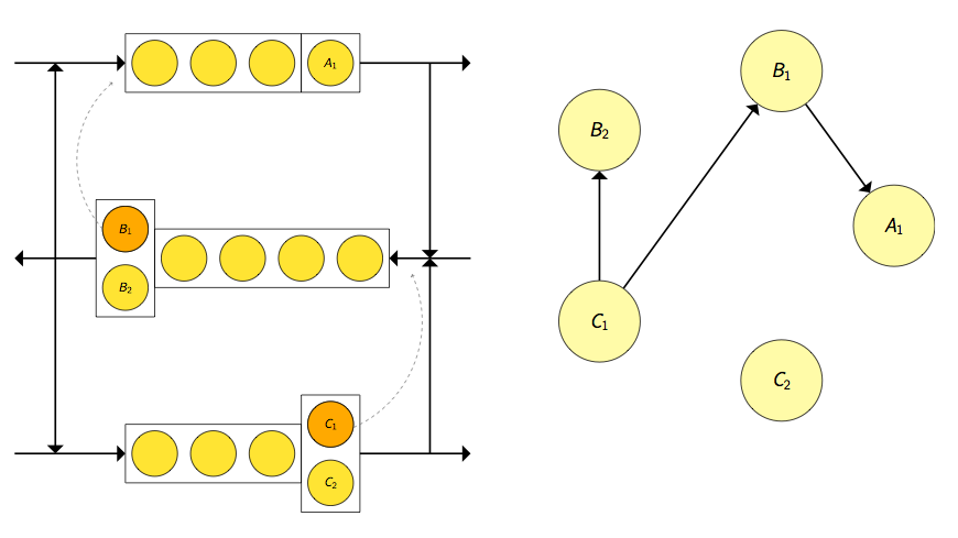
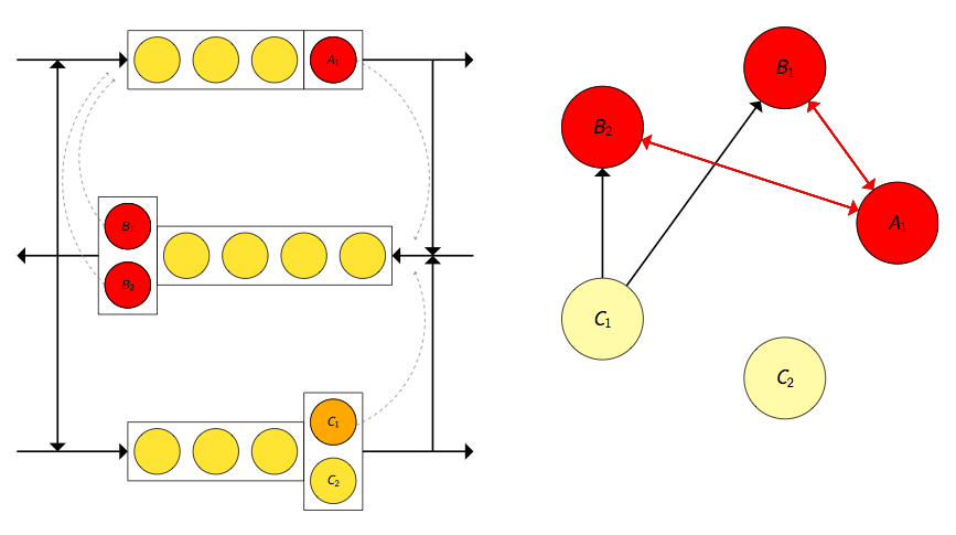
Now deadlock occurs if and only if \(D(t)\) contains a knot (an inescapable set of vertices). In the example below the knot and deadlocked servers are highlighted in red.
This result has been exploited as a deadlock detection mechanism in the Ciw library, a Python library developed by us and used in this project for simulating queueing networks.
Effects on the time to deadlock
Using the Ciw library the time until deadlock is reached from an empty system can be recorded. By building Markov chain models of simple deadlocking queueing networks the mean time to deadlock from an empty system can be estimated. We ran multiple scenarios to investigate the effect of varying the network parameters on the time to deadlock. In summary:
- Increasing the arrival rate of the system increases the time to deadlock (customers arrive quicker, so the queue fills up quicker).
- Increasing the queueing capacity decreases the time to deadlock (more customers can arrive before the capacity fills up).
- Increasing the number of servers decreases the time to deadlock (similar to queueing capacity, but a greater effect).
- Increasing the transition probabilities increases the time to deadlock (customers are less likely to leave the system, so more likely to get blocked).
The most interesting effect comes by varying the service rate \(\mu\). This produces the bowl like graph shown below.
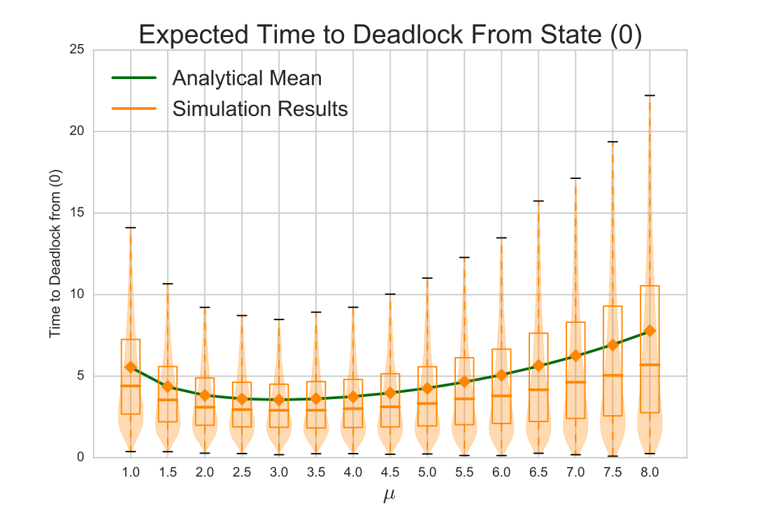
There seems to be some service rate threshold \(\hat{\mu}\) that yields the shortest time to deadlock. Although initially surprising, this does make sense, as services effect customers rejoining the queue and leaving the system, which have opposite effects on the time to deadlock:
- As \(\mu \rightarrow 0\), the mean service time approaches \(\infty\). Deadlock cannot occur as no customer leaves service to become blocked, so the time to deadlock approaches \(\infty\).
- If \(\mu < \hat{\mu}\), the arrival rate is relatively large compared to the service rate, and so the system is more than likely full. Here increasing the service rate increases the chance that a customer wants to rejoin the queue and thus become deadlocked. So the time to deadlock decreases as \(\mu\) increases.
- If \(\mu > \hat{\mu}\), the service rate is large enough that the system is probably not full. Now increasing the service rate increases the chance of a customer leaving the system, decreasing the chance of a blockage (as there are less customers in the queue). So the time to deadlock increases as \(\mu\) increases.
- As \(\mu \rightarrow \infty\) the mean service time approaches \(0\). A queue cannot build up as nobody spends time in service, therefore no blockages can occur, and the time to deadlock approaches \(\infty\).
Final word
This was my first proper research project I’ve worked on, and I enjoyed it very much. I particularly liked how this problem occurred to us in the first place: while implementing the blocking mechanism of restricted queueing networks in our discrete event simulation software (a precursor to Ciw), our automated testing suite kept failing.
For a while we obviously believed we had bugs in our code. Then looking a little closer at the tests, we realised our problem, the parameters we had chosen were causing the simulation to hit deadlock (not a concept I’d encountered at this point), and so skewing our performance measures. This then led to a very interesting and fruitful research project!