This week marks the first week back teaching, and I’m excited to teach one of my favourite modules Preliminary Mathematics II, where I introduce data and probability concepts to non-mathematics students. I always introduce the Normal distribution by saying “lots of natural things follow the Normal distribution, like human height”. This is something I’ve been repeating to students since learning it myself in school. But why does that happen?

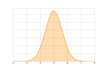
It’s nice to begin by talking about a Galton board (or bean machine) which shows that a small cumulative increments either side of a starting point results in a final resting place that follows a Normal distribution.

We could say that as a child’s height will differ by a small increment to their parents; then this Galton board can explain why human height follows a Normal distribution. But this seems to me a bit of a hand-wavy explanation.

Let’s think about Darwin’s theory of natural selection.

Darwin’s model

It is well known that parents pass on attributes to their offspring, usually by producing some sort of “average” of the parents. Now Darwin believed that all attributes seen today (ignoring mutations) existed as a large population in the past, and only the fittest survived today. I want to find out why what survives today seems to follow a Normal distribution.

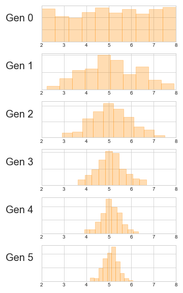
So, I simulated a diverse population of ‘heights’. Each generation I randomly paired up some parents, who produce two offspring whose attributes are the average of the parents’ heights:

>>> import random

>>> def next_gen_darwin(gen):
...     new_gen = []
...     random.shuffle(gen)
...     for i in range(len(gen)):
...         if i % 2 == 0:
...             g1 = (gen[i] + gen[i+1]) / 2
...             g2 = (gen[i] + gen[i+1]) / 2
...             new_gen.append(g1)
...             new_gen.append(g2)
...     return new_gen

Now imagine our starting population has uniformly random heights between 2 foot and 8 foot. Simulate six generations:

>>> random.seed(0)
>>> gens = [[random.uniform(2,8) for _ in range(500)]]
>>> for generation in range(6):
...     gens.append(next_gen_darwin(gens[-1]))

Plotting the distribution of heights of each generation show that they begin to approach a Normal distribution:

Why does this happen? Let’s recall the Central Limit Theorem:

The Central Limit Theorem roughly states that when random samples of \(n\) independent random variables are summed, their sums follow a Normal distribution as \(n \to \infty\).

Consider the \(k^{\text{th}}\) generation:

• This is the distribution of sums of random¹ samples of size \(2\) of the previous generation (divided by \(2\)),
• In turn this is the sum of random samples of size \(2^k\) of the first generation (divided by \(2^k\)),

and so the Central Limit Theorem can be applied: as the generation \(k\) increases, the distribution of heights should approach the Normal distribution (fairly quickly), explaining that often said phenomenon that human height follows a Normal distribution.

“But wait!” I hear you shout, “It’s 1858 and Darwin’s Origin of the Species hasn’t been published yet!” Does Lamarck’s theory also fit?

Lamarck’s model

Before Charles Darwin, it was Jean-Baptiste Lamarck’s theory that dominated. Lamarck also believed that parents pass their attributes on to their offspring. However he believed instead of all possible variation existing at the beginning, that species began with homogeneous attributes and individuals can change those attributes over the course of their lives, and pass these new acquired attributes to their offspring.

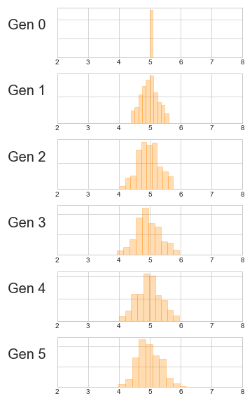
So, I simulated a homogeneous population of ‘heights’. Each generation I randomly paired up some parents, they each acquire some height attribute (their height increases by a value uniformly distributed between \(-\epsilon\) and \(\epsilon\)). They produce two offspring whose attributes are the average of the parents’ acquired heights:

>>> def next_gen_lamarck(gen, epsilon):
...     new_gen = []
...     random.shuffle(gen)
...     for i in range(len(gen)):
...         if i % 2 == 0:
...             parent1 = gen[i] + random.uniform(-epsilon, epsilon)
...             parent2 = gen[i+1] + random.uniform(-epsilon, epsilon)
...             g1 = ((parent1 + parent2) / 2)
...             g2 = ((parent1 + parent2) / 2)
...             new_gen.append(g1)
...             new_gen.append(g2)
...     return new_gen

Now imagine our starting population has height exactly 5 foot. Simulate six generations (with \(\epsilon = 0.7\)):

>>> random.seed(0)
>>> gens = [[5.0 for _ in range(500)]]
>>> for generation in range(6):
...     gens.append(next_gen_lamarck(gens[-1], 0.7))

Plotting the distribution of heights of each generation show that they also begin to approach a Normal distribution:

Again, consider the \(k^{\text{th}}\) generation:

• This is the distribution of sums of random samples of size \(2\) of the previous acquired generation (divided by \(2\)),
• The previous acquired generation is the sum of elements of the original previous generation and \(x \sim \text{Uniform}(-\epsilon, \epsilon)\),
• So, in turn, the \(k^{\text{th}}\) generation is the sum of random samples of size \(2^k\) of elements of the first generation (constants of 5) plus \(kx\) (and divided by \(2^k\)), where \(x \sim \text{Uniform}(-\epsilon, \epsilon)\),

and so the Central Limit Theorem can be applied again, explaining the trend towards normality.

Remarks

The analysis in the post doesn’t really explain why human height is Normally distributed, as the models are oversimplified. However it has given me a greater understanding of the phenomenon, and so greater confidence in chatting about it in class.