I had a disagreement with my Grampa this weekend. He insists ‘old money’ (pre-decimalisation) is much simpler than our current decimalised system. And I find it so confusing! I thought, there must be a away of measuring this.

I’ll consider three coinage systems here (as fractions of their largest coin):

• ‘Old money’, that is British pound sterling pre-decimalisation with the following coins: penny (1d), threepence (3d), sixpence (6d), shilling (12d), florin (24d), half crown (30d), crown (60d), and sovereign (£1 or 240d);¹
• Euros (or British pound sterling post-decimalisation, as they have the same denominations) with the following coins: 1c, 2c, 5c, 10c, 20c, 50c, and €1 or 100c;
• American dollars with the following coins: cent (1¢), nickel (5¢), dime (10¢), quarter (25¢), half-dollar (50¢), and a dollar ($1 or 100¢).

I’ll compare these in three dimensions: efficiency, availability, and complexity. I’ll use brute-force to evaluate these, using Python’s itertools and pandas to analyse all possible coin combinations below the value of the currencies’ largest coin.

Efficiency

A common mathematical puzzle in coins is the change-making problem. That is, for a given value of money, what is the minimum number of coins needed to make this value. This can usually be solved using linear programming or dynamic programming, but I use a brute force approach here. For all possible values under their largest coin, we get:

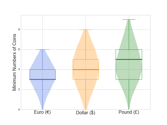
Euros are by far the most efficient currency with pre-decimalised British money being the least efficient.

Availability

Here I wanted to measure the currencies’ robustness to running out of a certain denomination, and began to consider the well known mathematical puzzle of the Frobenius coin problem (also known as the McNugget problem), when certain denominations were removed from the set. This is a hard problem, though could be brute-forced in this case.

I simplified the problem by asking a similar question of what percentage of all possible values am I able to make out of \(n\) coins? We get:

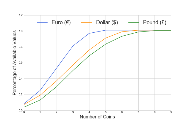
Euros have a much higher availability than dollar, which in turn are more available than pre-decimalised British coins.

Complexity

What did my Grampa originally mean by ‘simpler’? I’m not too sure, but we can measure complexity by considering coinage as a probabilistic problem: assume there are \(\left\lfloor\frac{x_\text{max}}{x_i}\right\rfloor\) of each denomination \(x\), where \(x_\text{max}\) is the value of the maximum coin. This corresponds to all possible obtainable values less than \(x_\text{max}\). Let \(N\) and \(V\) be random variables representing a randomly chosen number of coins and a randomly chosen value to obtain, respectively. Let \(\mathbb{P}(N=n, V=v)\) be the probability of getting a value of \(v\) with \(n\) randomly chosen coins.

We can measure the Shannon entropy of each marginal distribution:

This can be thought of kind of like a measure of variance, but for nominal data (nominal here because we don’t care how far away the values/numbers of coins are, just that they are different).

We get:

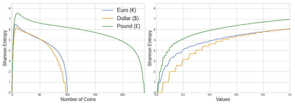
Here the American dollar is the least complex currency, closely followed by the Euro. Pre-decimalised British coins display the largest amount of complexity of the three.

We can also measure the joint entropy of the distribution:

Measured jointly, Euros come out as the simplest currency (just) with \(H(N, V) = 11.44\), then American dollars with \(H(N, V) = 11.53\), and finally pre-decimalised British coins with \(H(N, V) = 13.40\).

Overall pre-decimalised British coins are the least efficient, least available, and most complex of the three currencies compared, justifying my confusion.

What about Gringotts?

JK Rowling invented quite odd currency denominations parodying the complexity of pre-decimalised British money. So I thought I’d also compare this.

• Wizarding money consists of knuts, sickles, and galleons, with 29 knuts to the sickle, and 17 sickles to the galleon.

In comparison to the other three:

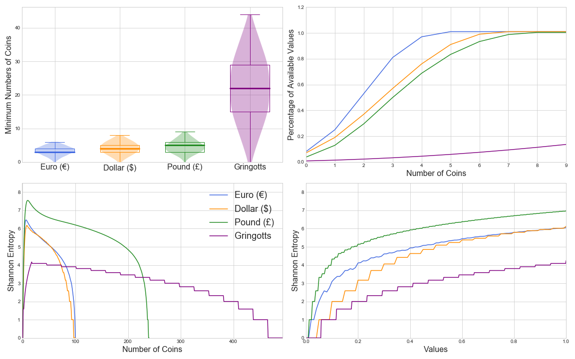
This is interesting! Wizarding money requires much more coins (so less efficient), and has a far lower availability than all three other currencies compared. However it has substantially lower marginal entropies (although a relatively moderate join entropy, \(H(N, V) = 12.12\)).

Why does wizarding money act to differently to the other coins? There is one major difference between wizarding money and the other three compared here: all denominations of wizarding money are multiples of the others. The other systems have at least one pair of denominations that are not multiples: dimes and quarters (10¢ and 25¢), 20c and 50c, and a number in old British money, e.g. florins and half crowns (24d and 30d). This may be one cause of a coinage’ complexity. It could also be a clue if trying to identify between real and fictional currencies.