Moving Averages with Irregular Gaps
At the moment Pandas doesn’t have a nice capabiliy to take moving averages of time series with irregular gaps, especially with the time data isn’t in datetime format. The traces library does. I’ll demonstrate with an example from Ciw.
Consider an M/M/c queue with a server schedule of 1 server for three days, and 2 servers for four days, running for four years:
>>> import ciw
>>> N = ciw.create_network(
...     arrival_distributions=[ciw.dists.Exponential(rate=5)],
...     service_distributions=[ciw.dists.Exponential(rate=7)],
...     number_of_servers=[[[1, 3], [2, 7]]]
... )

>>> ciw.seed(0)
>>> Q = ciw.Simulation(N, tracker=ciw.trackers.SystemPopulation())
>>> Q.simulate_until_max_time(365 * 4)
Here a state tracker is used to track the systems state over time. It records the entire history of the state changes, that is an irregularly spaced time-series:
>>> Q.statetracker.history
[[0.0, 0],
 [0.3721214222130447, 1],
 [0.48126405132136324, 2],
 [0.541192513764126, 3],
 [0.5747827297804392, 2],
 [0.6489374706664274, 1],
 [0.6843834637175561, 2],
 [0.7566671923851261, 3],
 ...
Plotting this doesn’t give us much insight, as it’s too stochastic:
>>> plt.plot(
...     [t[0] for t in Q.statetracker.history],
...     [t[1] for t in Q.statetracker.history],
...     c='black'
... )
>>> plt.xlabel('Days')
>>> plt.ylabel('Customers')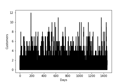
The traces library let’s us take moving averages over this irregular time series, with any window size we want, e.g. a 7-day moving average, 30-day moving average, or a quarterly moving average:
>>> import traces
>>> series = traces.TimeSeries()
>>> for timestamp, state in Q.statetracker.history:
...     series[timestamp] = state

>>> series_ma7 = series.moving_average(7, pandas=True)
>>> series_ma30 = series.moving_average(30, pandas=True)
>>> series_maQ = series.moving_average(365/4, pandas=True)

>>> series_ma7
0.0       1.164410
7.0       0.805528
14.0      1.780030
21.0      1.076819
28.0      1.224057
            ...
1428.0    0.834888
1435.0    0.966756
1442.0    2.827261
1449.0    1.074443
1456.0    0.775233
Length: 209, dtype: float64
This gives us something more interpretable:
>>> plt.plot(series_ma7, c='black', alpha=0.3, label='7 day MA')
>>> plt.plot(series_ma30, c='black', linestyle='dotted', label='30 day MA');
>>> plt.plot(series_maQ, c='black', label='Quarterly MA');
>>> plt.legend()
>>> plt.xlabel('Days')
>>> plt.ylabel('Customers')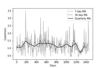
The traces library also allows us to do this from file, which I think is a bit nicer:
>>> Q.write_records_to_file('records.csv')

>>> series = traces.TimeSeries.from_csv(
...     filename="records.csv",
...     time_column=3,  # Arrival dates
...     time_transform=float,
...     value_column=4, # Waiting times
...     value_transform=float
... )

>>> series_wait_ma = series.moving_average(30, pandas=True)

>>> plt.plot(series_wait_ma, c='black')
>>> plt.xlabel('Days')
>>> plt.ylabel('Waiting Time')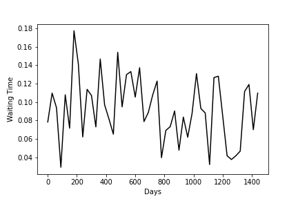
When taking a moving average we can return a pandas Series, which makes this nice and compatible with other analyses too. This library is much nicer than my previous soluiton of converting to datetime and back!