This will be a guide in how to build DES+SD hybrid simulations with Ciw. These hybrid simulations are models that combine the discrete time methodology of discrete event simulation (DES), and the continuous time methodology of systems dynamics (SD). I wrote a paper with a masters student, Yawen Tian, a couple of year ago explaining how this is possible in Python using the Ciw and SciPy libraries, explaining the methodology, model architectures, synchronicity issues, and some examples: “Implementing hybrid simulations that integrate DES+SD in Python”. In that paper we show that the main part the method is to solve the differential equations of the SD component in between each discrete event of the DES component, updating all parameters at all points. Here, through an example, I want to focus on the steps we took to adapt the Ciw source code to build these models, as a guide for students or others wanting to reproduce the work.

You will need:

Some knowledge of discrete event simulation
Some knowledge of systems dynamics
To have read the above paper
Python (guaranteed to work on version 3.7)
Ciw (guaranteed to work on version 2.3.5)
SciPy (guaranteed to work on version 1.7.3)

Problem

Amazon Kindle add a lot of books to their store every day. There is a certain probability that these books contain some errors. Once on sale on the Kindle store, readers can report errors. These error reports join a queue and are corrected by a set number of staff. When not correcting errors, staff work at finding the errors and correcting errors in the books on the Kindle store.

It takes a staff member between 1 and 2 hours, Uniformly distributed, to correct an error. Errors are reported randomly at a rate of \(r\), and join the queue for correction according to an Exponential distribution.

How many staff should the Kindle store hire to do this job?

Step 1 - Formulation

Why is a hybrid DES+SD model appropriate here? At first, we don’t see any continuous time elements, and the whole system could be modelled using a DES only. However, the numbers of books and errors involved are quite large, and this could take a huge amount of computer memory and very long time to run. So SD might be better. Looking at the level of detail required, there is a queue involved with integer numbers of error reports and integer number of servers, so this component makes sense to model as a DES. For everything else, they are described in rates, may be large in number or frequency, and not much detail is required, and so could be modelled as SD. Therefore, these will be the two components.

We can see that the components are very integrated - stock levels and rates from the SD affect the DES queue (e.g. numbers of books with errors in them affecting the arrival rate to the queue), and details from the DES affect the SD (e.g. numbers of free servers affect the rate of change in numbers of books). So an integrated DES+SD is required. In the language used in the paper above: the DES queue component lives within a world described by SD, and so we have a \(DES \subset SD\) system.

Let’s formulate the model:

Let \(B_0\), \(B_1\), \(B_2\) and \(B_3\) represent the numbers of books with 0, 1, 2, and 3 errors respectively (B),
let \(T\) represent the total number of errors, where \(T = \max(B_1 + 2B_2 + 3B_3, 1)\), ensuring there is never zero errors (total_errors),
let \(\eta\) represent the rate at which new books are added to the store (new_book_rate),
let \(p\) be the probability that a book has one error (prob_error),
let \(r\) be the rate at which readers report errors (report_rate),
let \(s\) be the rate at which staff report errors (search_rate),
let \(\Lambda\) be the rate at which errors get reported (rate),
let \(c\) the be number of staff (number_of_servers),
let \(c_f\) be the number of staff free to find and correct errors themselves (free_staff).
We will assume that the number of errors per book follows a (truncated) geometric distribution, so letting \(p_i\) be the probability that a book has \(i\) errors, then \(p_i = \frac{(1 - p)p^i}{1 - p^4}\) (ps).

We can draw the relationships as a queueing/stock-and-flow diagram as follows:

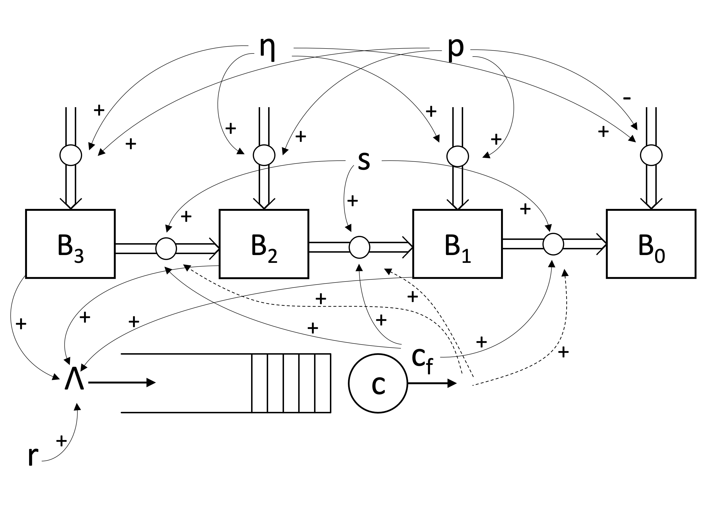
From this we can write down the system differential equations that describe the SD component:

\[\begin{align*} \frac{dB_0}{dt} &= p_0 \eta + \frac{s c_f}{T} B_1\\ \frac{dB_1}{dt} &= p_1 \eta + \frac{s c_f}{T} (B_2 - B_1)\\ \frac{dB_2}{dt} &= p_2 \eta + \frac{s c_f}{T} (B_3 - B_2)\\ \frac{dB_3}{dt} &= p_3 \eta - \frac{s c_f}{T} B_3 \end{align*}\]

The DES component is a single queue with \(c\) servers, and three classes of customer. Customers are error reports, and each class represents errors from books with 1, 2 or 3 errors in them. Each class’s inter-arrival times are Exponentially distributed with arrival rate \(\Lambda_i = irB_i\). It takes between 1 and 2 hours Uniformly to correct an error. The parameter \(c_f\) is dynamic and calculated from the DES component.

Furthermore, upon correcting an error (completing a service) of type \(i\), we take 1 away from \(B_i\) and add 1 to \(B_{i-1}\). This represents a book losing one of its errors.

Step 2 - Write the SD Component

Now we have defined all the relationships, we can write the SD component. This will be a class with three methods: __init__; differential_equations; and solve.

__init__: this takes in arguments and sets attributes corresponding to the parameters and variables above. An important part here is to also define an attribute time, this is NumPy array of time points over which we will have numerically solved the differential equations. For now, nothing has been solved yet, so we set this to just be a vector containing zero.

  import numpy as np
  from scipy.integrate import odeint
  
  class SD():
      """
      A class to hold the SD component.
      """
      def __init__(
          self,
          initial_number_of_errors,
          new_book_rate,
          prob_error,
          report_rate,
          search_rate,
          **kwargs
      ):
          """
          Initialised the parameters for the SD component
          """
          p = prob_error
          self.ps = [(1 - p) * (p ** i) / (1 - (p ** (4))) for i in range(4)]
          self.B = [[initial_number_of_errors * pi] for pi in self.ps]
          self.new_book_rate = new_book_rate
          self.report_rate = report_rate
          self.search_rate = search_rate
          self.time = np.array([0])

Note here self.B is a list containing four lists, each representing the values of \(B_0\), \(B_1\), \(B_2\) and \(B_3\) over the time domain. We have currently filled them with the initial values at time 0, that is \(p_i\) multiplied by initial_number_of_errors.

differential_equations: this takes in the current vector of \(B_i\)s, the time domain, and some other arguments that will change according to the DES component, and returns the four instantaneous derivatives defined above.

      def differential_equations(self, y, time_domain, free_staff):
          """
          Defines the differential equations that define the system.
          Returns the value of the derivatives for each B_i.
          """
          B0, B1, B2, B3 = y
          total_errors = max(B1 + (2 * B2) + (3 * B3), 1)
          dB0dt = (self.ps[0] * self.new_book_rate) + (self.search_rate * free_staff * ((B1) / total_errors))
          dB1dt = (self.ps[1] * self.new_book_rate) + (self.search_rate * free_staff * ((B2 - B1) / total_errors)  )
          dB2dt = (self.ps[2] * self.new_book_rate) + (self.search_rate * free_staff * ((B3 - B2) / total_errors)  )
          dB3dt = (self.ps[3] * self.new_book_rate) + (self.search_rate * free_staff * ((-B3) / total_errors))
          return dB0dt, dB1dt, dB2dt, dB3dt

Here y is a vector of the initial values (their values at the time of the last discrete event) of \(B_0\), \(B_1\), \(B_2\) and \(B_3\). The method corresponds exactly with the differential equations defined above. The time_domain argument will be a NumPy array corresponding to the time points over which we will solve these differential equations, that is from the time of the last discrete event to the current time. It is unused in be the method, but required in order for SciPy to numerically solve the equations. There is one additional argument: free_staff (\(c_f\)). This will come from the DES component, so we won’t worry about where is has come from yet.

solve: this uses the SciPy library to solve the differential equations between the discrete events of the DES component.

    def solve(self, t, **kwargs):
        """
        Solves the differential equations from
        the time of the pervious event to time t.
        """
        leaving_class = kwargs['leaving_class']
        free_staff = kwargs['free_staff']
          
        # Solve the SD over the relevant time domain
        y = (self.B[0][-1], self.B[1][-1], self.B[2][-1], self.B[3][-1])
        relevant = (self.time_domain <= t) & (self.time_domain >= self.time[-1])
        times_between_events = np.concatenate(
            (np.array([self.time[-1]]), self.time_domain[relevant], np.array([t])),
            axis=None
        )
        results = odeint(
            self.differential_equations,
            y,
            times_between_events,
            args = (free_staff,)
        )
          
        B0, B1, B2, B3 = results.T
        self.B[0] = np.append(self.B[0], B0)
        self.B[1] = np.append(self.B[1], B1)
        self.B[2] = np.append(self.B[2], B2)
        self.B[3] = np.append(self.B[3], B3)
          
        # Add and subtract the current error from it's pool
        f = [1 if i == leaving_class else 0 for i in range(3)]
        self.B[0][-1] = self.B[0][-1] + f[0]
        self.B[1][-1] = max(self.B[1][-1] + f[1] - f[0], 0)
        self.B[2][-1] = max(self.B[2][-1] + f[2] - f[1], 0)
        self.B[3][-1] = max(self.B[3][-1] - f[2], 0)

        # Update the times over which we've already solved the SD
        self.time = np.append(self.time, times_between_events)

The main point of this method is to use SciPy’s odeint function to numerically solve the differential equations from the time of the last discrete event (self.time[-1]), to the current time (the argument t). This is the relevant time domain (or the times_between_events when including the endpoints). They are calculated by taking slices of self.time_domain, as yet undefined, which should be a vector of equally spaced time points from 0 to the maximum simulation run time.

After solving the SD between the events, we then remove the currently corrected error from the relevant pool of errors. We do this by adding or subtracting from the last value in each vector of self.B.

Notice that to do all this, we need two arguments: leaving_class and free_staff. These are given to the function through keyword arguments. Again, we do not know how these are calculate yet, that is the job of the DES component.

Step 3 - Understand how the SD and DES Components Talk to Each Other

Now we need to think about which events of the DES component will affect the parameters of the SD component, and which events of the DES need information from the SD component. These are the events in between which we will solve the SD components. In this case we have:

Releasing individuals - When releasing an individual, we have to update the SD component by moving an error from one pool, \(B_i\), to the next, \(B_{i-1}\). This will effect Ciw’s node object.
Sampling arrivals - The arrival distributions rely on parameters from the SD component, and so when we sample arrivals we need to make sure we have the most up-to-date parameters from the SD component. This will effect Ciw’s distribution object.

In addition to these, we also have to solve the SD right at the end of the simulation, between the final event and the end simulation time.

Step 4 - Write a Template for the DES Component

First we will write a generic simulation object that includes the SD component that we have just written. This inherits from Ciw’s Simulation class, adding appropriate attributes and methods to talk to the SD component.

Note that we might need to re-write this later to ensure all the correct information is being passed to each object, but for now:

import ciw

class HybridSimulation(ciw.Simulation):
    """
    A Simulation object that includes the SD component as an
    attribute and communicates with it at the relevant points
    of the simulation.
    """
    def __init__(self, network, **kwargs):
        """
        Initialises the HybridSimulation object.
        Creates and attaches the SD component.
        """
        self.SD = SD(**kwargs)
        super().__init__(network=network, node_class=HybridNode)
        
    def simulate_until_max_time(self, max_simulation_time, n_steps):
        """
        Runs the simulation until the max_simulation time.
        Creates the time domain, runs the simulation, and solves
        the SD component one last time.
        """
        self.SD.time_domain = np.linspace(0, max_simulation_time, n_steps)
        super().simulate_until_max_time(max_simulation_time)
        self.SD.solve(
            t=max_simulation_time,
            leaving_class=None,
            free_staff=None
        )

The __init__ method is overwritten. This adds the an instance of the SD class as an attribute. It also ensures that we use a HybridNode (yet to be defined) is used instead of Ciw’s usual node class.
The simulate_until_max_time method is overwritten. First, a time_domain attribute is given to the SD component. This is an array of n_steps equally spaced time points between 0 and the max_simulation_time. Then, after the simulation is run, the SD component is solved one last time from the last event to max_simulation_time.

Step 5 - Complete Writing the DES Component

We identified two events where the DES component needed to interact with the SD component: releasing individuals, and sampling inter-arrival times. Let’s take them in turn:

Releasing individuals: First, in order to solve the SD component, we need to pass it free_staff, which represents the number of staff that were free since the last event. Therefore, the first thing we should do is make a new HybridNode object, that inherits from Ciw’s Node object, and keeps track of how many servers are free (we will have to initially set this attribute from the start of the simulation later on):

class HybridNode(ciw.Node):
    """
    A Node object that communicates with the SD component at
    the relevant points of the simulation.
    """
    def update_free_staff(self):
        """
        Updates the `free_staff` attribute with the number
        of staff that are currently free.
        """
        self.free_staff = sum(not s.busy for s in self.servers)

Now we need to overwrite the release method so that it solves the SD component. There is one more thing we need: the leaving_class, the class of the customer currently leaving. We can get this in the first line of the method below. Then we release as usual, solve the SD, then update the number of free staff.

    def release(self, next_individual_index, next_node):
        """
        Releases the current individual at the end of their service.
        Solves the SD component.
        """
        leaving_class = self.all_individuals[next_individual_index].customer_class
        super().release(next_individual_index, next_node)
        self.simulation.SD.solve(
            t=self.get_now(),
            leaving_class=leaving_class,
            free_staff=self.free_staff
        )
        self.update_free_staff()

Now, remember we said that we’d need to set the node’s free_staff attribute at the beginning of the simulation run. So we add a line doing that to the simulate_until_max_time method from Step 4, and then pass that to the SD solve. So the HybridSimulation class now becomes:

class HybridSimulation(ciw.Simulation):
    """
    A Simulation object that includes the SD component as an
    attribute and communicates with it at the relevant points
    of the simulation.
    """
    def __init__(self, network, **kwargs):
        """
        Initialises the HybridSimulation object.
        Creates and attaches the SD component.
        """
        self.SD = SD(**kwargs)
        super().__init__(network=network, node_class=HybridNode)
          
    def simulate_until_max_time(self, max_simulation_time, n_steps):
        """
        Runs the simulation until the max_simulation time.
        Sets the `free_staff` attribute, creates the time
        domain, runs the simulation, and solves the SD
        component one last time.
        """
        self.nodes[1].free_staff = self.nodes[1].c
        self.SD.time_domain = np.linspace(0, max_simulation_time, n_steps)
        super().simulate_until_max_time(max_simulation_time)
        self.SD.solve(
            t=max_simulation_time,
            leaving_class=None,
            free_staff=self.nodes[1].free_staff
        )

Sampling inter-arrivals:

When sampling an inter-arrival time for customers of class \(i\), the arrival rate is \(\Lambda_i = irB_i\), and so we need the latest information from the SD component. So before sampling an inter-arrival time we have to solve the SD component. This will happen within the distribution object. So we can make a new distribution class by inheriting from Ciw’s generic distribution class.

Now as we have three classes of customer, each with a slightly different arrival rate. So we need three different Distribution object. We will do this by defining it within a function, returning a different object for each \(i\):
```
def get_arrival_distribution(i):
    """
    Creates a distribution class and returns and instance of that class.
    Creates a distribution class for arrivals from B_i.
    Solves the SD component before sampling.
    """
    class SolveSDArrivals(ciw.dists.Distribution):
        def sample(self, t=None, ind=None):
            if t > 0:
                self.simulation.SD.solve(
                    t=t,
                    leaving_class=None,
                    free_staff=self.simulation.nodes[1].free_staff
                )
            rate = self.simulation.SD.B[i][-1] * i * self.simulation.SD.report_rate
            return ciw.dists.Exponential(rate).sample()
    return SolveSDArrivals()
```
Just like other custom distributions, we just need to overwrite the sample method. First we solve the SD component, then calculate the rate by accessing the parameters from the SD component, and then sample from an Exponential distribution using that rate.

Step 6 - Bringing it All Together and Defining the System

Now we have all the classes in place to define the Network, build the hybrid simulation object, and run. Below is the system with 8 staff members, 200 total errors in the pool to begin with, \(\eta = 100\), \(p = 0.1\), \(r = 1\), \(s = 0.4\). Time units are in days.

N = ciw.create_network(
    arrival_distributions={
        'Class 0': [get_arrival_distribution(1)],
        'Class 1': [get_arrival_distribution(2)],
        'Class 2': [get_arrival_distribution(3)]},
    service_distributions={
        'Class 0': [ciw.dists.Uniform(1/24, 2/24)],
        'Class 1': [ciw.dists.Uniform(1/24, 2/24)],
        'Class 2': [ciw.dists.Uniform(1/24, 2/24)]},
    number_of_servers=[8]
)

Q = HybridSimulation(
    network=N,
    initial_number_of_errors=200,
    new_book_rate=100,
    prob_error=0.1,
    report_rate=1,
    search_rate=0.4
)

Step 7 - Running the Simulation and Finding Results

Now we can run it for 6 weeks. We have chosen to solve the SD component in time steps of \(100^{th}\) of a day.

n_weeks = 6
Q.simulate_until_max_time(
	max_simulation_tim=n_weeks * 7,
	n_steps=n_weeks * 7 * 100
)

Once it’s run, we can inspect the DES or SD components for the results. E.g., here we get the total number of errors over the time domain:

total_errors = Q.SD.B[1] + (2 * Q.SD.B[2]) + (3 * Q.SD.B[3])    

In order to smooth out any variability caused by the randomness, we should run many trials and take averages. Using Pandas or NumPy we can take averages over the trials for each time step in the time domain. This allows for smoothed time series results.

Experiments

Now that the hybrid simulation is built and we know how to run it, we can use it to gain some insights into the system in question. Here are two examples:

First we might like to know, for a given set of parameters, if the total number of errors reaches a steady state, or increases uncontrollably. We can look at the average total_errors over time. We can compare this for different values of \(r\) and different values of \(c\). All other parameters remain as above. Plotting averages over 18 trials and taking rolling means we get:

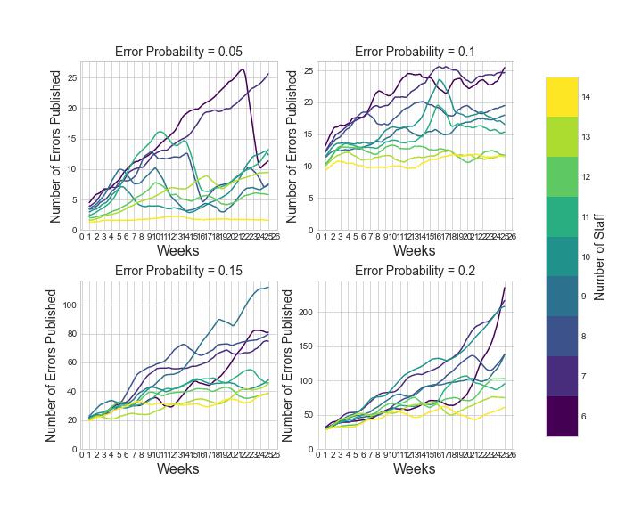
When \(r=0.05\) the total number of errors remains stable, albeit with high variability, for all numbers of staff modelled. However, the value for which it remains stable decreases as the number of servers increase. As \(r\) increases, these stable values also increase. However we also see, that there are some combinations of \(r\) and \(c\) where the total number of errors doesn’t remain stable, but increases uncontrollably - for example \(r=0.2\) and \(c=6\). From the patters shown, we might hypothesise that the threshold for the number of servers required for stability increases as \(r\) increases.

Next we’ll fix \(r\) and investigate the total number of errors after 8 weeks as we increase the number of staff. The box and violin plots show the distribution of the total number of errors over 50 trials, and the line shows the mean over the trials:

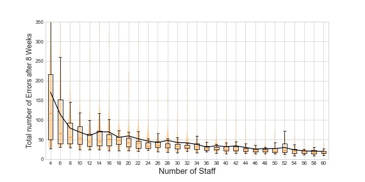
We see that there is a sharp drop in numbers of errors up to \(c = 12\), and then a shallower drop thereafter. This might show that when \(c \leq 12\) the system has not reached a steady state and the number of reported errors is increasing in the queue; but when \(c > 12\) the system has reached steady state, and the excess number of staff are hard at work finding and correcting errors in their free time, thus still reducing the overall number of errors in the pool after 8 weeks. Amazon Kindle can then decide, if they would like less than 50 errors in the pool after 8 weeks, then they need to employ at least 30 members of staff.

All code used to create this guide is available at: https://github.com/geraintpalmer/KindleErrors.