Instructions

• Please look over this worksheet before coming to the session:
  • Either work through this worksheet before the session, and bring any difficulties / problems to the session so that we can look them over together.
  • Or work through the worksheet in the session, addressing any difficulties when you get to them.

• Anything you wish to go over that isn’t covered in this worksheet, please bring examples and we can work through them together.

• I recommend using Overleaf, a web based tool for writing and compiling \(\TeX\) files. It’s great for learning \(\LaTeX\). Feel free to use whatever you are comfortable with. Note that the free accounts on Overleaf have a limit, and so I recommend obtaining a local version of LaTeX for serious work.

Contents

• 1. Basics
• 2. Sections
• 3. Lists & Tables
• 4. Mathematics
• 5. Figures
• 6. Labels
• 7. Code
• 8. Environments
• 9. Bibliographies
• 10. Presentations

1. Basics

Many LaTeX commands begin with a backslash \. Anything beginning with % are comments and are ignored. We need to tell the compiler which document class we are using (an article in this case). Then we need to tell LaTeX where the document itself begins and where it ends:

\documentclass{article}

\begin{document}
% Your contents here...  
\end{document}

Code between \begin and \end document is called the main body. Code that precedes \begin{document} is called the preamble. Here is where declaration on which packages to use are written. It is also where title information can be given:

\title{My awesome title}
\author{G Palmer}
\date{28/9/2016}

We can automatically yield today’s date with \today. Then to produce the title, in the main body of the document, we declare that we wish to make a title:

\begin{document}
\maketitle
\end{document}

Many articles have an abstract, which briefly outlines the contents of the article. Within the main body, we can create an abstract using:

\begin{abstract}
% Your abstract here...
\end{abstract}

Challenge: Create an article with a title, author, date, and abstract.

2. Sections

Section are useful for organising your article into manageable chunks for reading. These are easily implemented in LaTeX:

\section{Turtles}
% Contents about turtles here...

\section{Clocks}
% Contents about clocks here...

Notice that section numbering is automatic, so there is no need to include numbering in your sections’ titles. Subsections (numbered 2.1, 2.2, etc.) can be achieved with \subsection{}.

To place a table of contents at the beginning of your document, which automatically lists on which pages each section begins, the following command can be placed at the beginning of a document:

\tableofcontents

Challenge: Include three sections in your article, entitled ‘Food & Drink’, ‘Furniture’, and ‘Mathematics’. Under the Food & Drink section, include the subsections ‘Fruit’, and ‘Vegetables’. Under the ‘Fruit’ subsection, include two further subsections entitled ‘Citrus Fruit’, and ‘Berries’. Experiment with further sectioning.

3. Lists & Tables

Bullet lists, numbered lists, and tables are convenient ways of displaying content. Bullet lists can be created using itemize, and items placed into the list using \item. An example is shown below:

\begin{itemize}
  \item Dalek
  \item Cyberman
  \item Weeping angel
\end{itemize}

For numbered lists, use enumerate:

\begin{enumerate}
  \item Dalek
  \item Cyberman
  \item Weeping angel
\end{enumerate}

Lists may be nested, and mixtures of itemize and enumerate may be used:

\begin{itemize}
  \item Companions
  \begin{enumerate}
    \item Rose
    \item Martha
    \item Donna
  \end{enumerate}
  \item Monsters
  \begin{itemize}
    \item Dalek
    \item Cyberman
    \item Weeping angel
  \end{itemize}
\end{itemize}

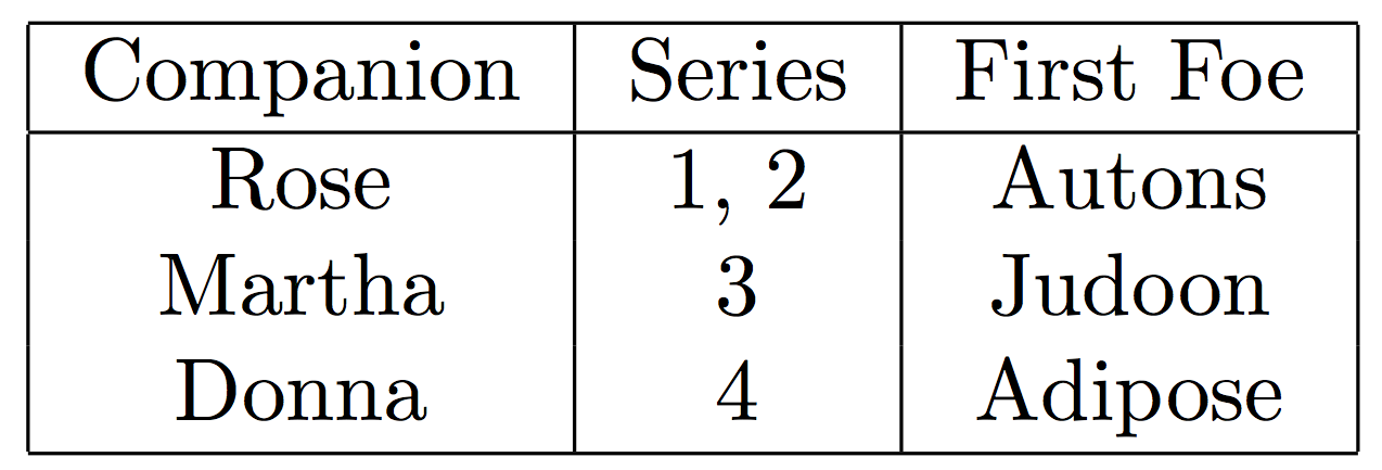
Tables are another way of organising content. This is achieved using tabular. Try to understand the example given below:

\begin{tabular}{|c|c|c|}
Companion & Series & First Foe \\
\hline
Rose & 1, 2 & Autons \\
Martha & 3 & Judoon \\
Donna & 4 & Adipose \\
\hline
\end{tabular}

The first line sets out the options for the table. We see there are three centred, c columns (try replacing these with r or l for right and left aligned columns). A | indicates a vertical drawn line before or between these columns. In the table environment itself we then insert contents row by row. A & indicates the end of a column, and to put further contents into the next column. A \\ denotes that the row has ended, and further contents should be in cells on the next row. Between rows, placing a \hline draws a horizontal line. Notice that in this simple example, each row must have 3 columns and 3 columns only, although we may add rows as we wish.

This yeids:

Further information on tables is available here.

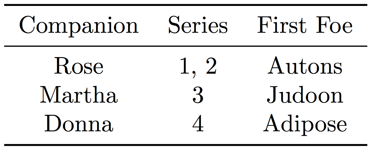
Tables can be made prettier by using the booktabs package. With this package vertical lines are not needed, and horizontal lines are resticted to \toprule, \midrule and bottomrule:

\usepackage{booktabs}

\begin{tabular}{ccc}
\toprule
Companion & Series & First Foe \\
\midrule
Rose & 1, 2 & Autons \\
Martha & 3 & Judoon \\
Donna & 4 & Adipose \\
\bottomrule
\end{tabular}

Compare this output with that above:

Challenge: Under the Furniture section create a numbered list of all the furniture in the room by size. Under each item, create an unordered list of some attributes of that piece of furniture. Experiment with further nesting.

Challenge: Under the Fruit section, create a table of 7 fruits, containing information on their colour, size, and shape. Experiment with different cell alignments, and cell borders.

4. Mathematics

Mathematics may be written in LaTeX in two ways, inline or in an equation environment. Inline mathematics like this \(y = mx + c\) may be achieved by wrapping the mathematics between two $ signs. However, if you wish to produce a separate equation, then use the the equation environment:

\begin{equation}
% Your mathematics here...
\end{equation}

Many simple mathematical operations in LaTeX are intuitive: +, -, =, >, <, and numbers and Latin letters are as you type them. Lower case Greek letters are produced by typing the letter after a backslash, \(\alpha\) is \alpha, and upper case letters simply capitalise the first letter, \(\Gamma\) is \Gamma. Some other useful symbols include:

• \(\neq\) is \neq
• \(\geq\) is \geq
• \(\leq\) is \leq
• \(\mathbb{R}\) is \mathbb{R}
• \(\mathbb{N}\) is \mathbb{N}
• \(\mathbb{Q}\) is \mathbb{Q}
• \(\mathbb{C}\) is \mathbb{C}
• \(\in\) is \in
• \(\int\) is \int
• \(\cup\) is \cup
• \(\propto\) is \propto
• \(\infty\) is \infty
• \(\rightarrow\) is \rightarrow

More of these symbols can be found here. Note that for some mathematical symbols and fonts, you may require the amsmath and amsfonts packages. Include them in your preamble:

\usepackage{amsmath}
\usepackage{amsfonts}

For accented characters simply apply a transformation to the relevant character, for example \(\hat{a}\) is \hat{a}, \(\bar{\beta}\) is \bar{\beta}. To raise to a power use ^, and to add an index use _, for example \(x^{4a - 2}\) is x^{4a - 2}, and \(W_{\alpha}\) is W_{\alpha}.

• Fractions are written using \frac{}{} with the nominator going in the first curly bracket, and the denominator going in the second curly bracket. Inline fractions may be written like \(1/2\) with 1/2.

• Brackets such as ( and [ need only be typed directly in LaTeX. Curly brackets ‘{‘ must be preceded by a backslash \{. These brackets do not adjust to the size of their contents. In order to do this precede left brackets with \left and right brackets with \right. Compare \((\frac{x^y}{a^b})\) with \(\left(\frac{x^y}{a^b}\right)\), produced with (\frac{x^y}{a^b}) and \left(\frac{x^y}{a^b}\right) respectively. \left and \right must come in pairs; if only one bracket is needed, replace the unneeded bracket with a ., e.g. \left[ a \right..

• In order to produce matrices, the pmatrix environment may be used (also look up matrix, bmatrix, vmatrix, etc, and also the array environment). The syntax is similar to that for tables. The following matrix may be produced using the code below:

  \[\begin{pmatrix}a & b \\ c & d\end{pmatrix}\]

  \begin{pmatrix}
  a & b \\
  c & d
  \end{pmatrix}
  

• Another environment, the align environment can be used to create equations aligned by the ‘=’ sign. For example the following piece of mathematics can be written using the code below:

  \[\begin{align}(x+2)(x-3)+6 &= x^2 -3x + 2x - 6 + 6\\ &= x^2 + x\\ &= x(x+1)\end{align}\]

  \begin{align}
  (x+2)(x-3)+6 &= x^2 -3x + 2x - 6 + 6\\
  &= x^2 + x\\
  &= x(x+1)
  \end{align}
  

  Similar to tables and matrices, \\ tells LaTeX there is a line break. We have also preceded all the = signs we wish to align with &.

• Piecewise equations can be written in LaTeX with an cases environment. Again, these have similar to syntax to matrices, arrays and tables. Study the following example of the Heavyside step function:

  \[H(x) = \begin{cases} 0 & x < 0\\\frac{1}{2} & x = 0\\1 & x > 0\end{cases}\]

  \begin{equation}
  H(x) =
    \begin{cases}
      0 & x < 0\\
      \frac{1}{2} & x = 0\\
      1 & x > 0
    \end{cases}
  \end{equation}
  

Challenge: Reproduce these in LaTeX:

1. \[\frac{\partial c}{\partial t} = D \nabla^2 \left( c^3 - c - \gamma \nabla^2 c \right)\]
2. \[H = \frac{1}{2} \int \left[ \sum_i \left( \frac{\partial \mathbf{S}}{\partial x_i} \right)^2 - J(\mathbf{S}) \right] dx\]
3. \[e = \lim_{n \rightarrow \infty} \left( 1 + \frac{1}{n} \right)^n\]
4. \[\mathbf{J} = \begin{bmatrix} \frac{d f_1}{d x_1} & \cdots & \frac{d f_1}{d x_n}\\ \vdots & \ddots & \vdots \\ \frac{d f_n}{d x_1} & \cdots & \frac{d f_n}{d x_n} \end{bmatrix}\]
5. \[\begin{align}(\theta-20)(\theta+6)+169 &= \theta^2 -20\theta +6\theta -120 + 169\\ &= \theta^2 - 14\theta + 49\\ &= (\theta - 7)^2\end{align}\]
6. \[\mathbb{E}_X \left[ g(X) \right] \geq g\left( \mathbb{E}_X [X] \right)\]

5. Figures

Figures may be added using the figure environment. This environment supports captions:

\begin{figure}
  % Your figure here...
  \caption{A brief description of the figure.}
\end{figure}

Pictures may be added using the graphicx package, and the command \includegraphics. This command takes in a width as an option, it is usual to state this in terms of the \textwidth. First include the package in the preamble:

\usepackage{graphicx}

Let’s add my_image.png, which we’ll put in the same folder as the main document, to be half the width of the text. Now we should get:

\begin{figure}
  \includegraphics[width=0.5\textwidth]{my_image.png}
  \caption{A brief description of the figure.}
\end{figure}

With the subcaption package subfigures can be places within figures. A subfigure environment works similar to the figure environment, allowing captions for both the subfigures and the overall figure:

\begin{figure}
  \begin{subfigure}{0.5\textwidth}
    \includegraphics[width=\textwidth]{my_image_1.png}
    \caption{A brief description of the first subfigure.}
  \end{subfigure}
  \begin{subfigure}{0.5\textwidth}
    \includegraphics[width=\textwidth]{my_image_2.png}
    \caption{A brief description of the second subfigure.}
  \end{subfigure}
  \caption{A caption for the whole figure}
\end{figure}

Challenge: Find an image of a piece of furniture on the internet, download it. Include it under the ‘Furniture’ section, add an appropriate caption.

We can create our own diagrams using the tikz package. This powerful package can be used to draw almost all diagrams you will require. We must include the package in the preamble:

\usepackage{tikz}

Basic manipulation includes drawing red a line between two coordinates (0, 0) and (0, 2):

\draw[draw=red] (0, 0) -- (0, 2);

drawing a blue circle of radius 5 with centre at coordinate (10, 20):

\draw[fill=blue] (10, 20) circle (5);

and placing text at a coordinate (4, 5):

\node at (4, 5) {Some text};

All tikz commands must end with a semicolon. The following flow diagram was drawn using the tikz code below:

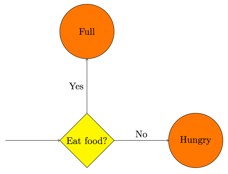
\begin{tikzpicture}
  \draw[->] (0, 0) -- (2, 0);
  \draw[fill=yellow] (2, 0) -- (3, 1) -- (4, 0) -- (3, -1) -- cycle;
  \node at (3, 0) {Eat food?};
  \draw[->] (3, 1) -- (3, 3) node[pos=0.5, left] {Yes};
  \draw[fill=orange] (3, 4) circle (1) node {Full};
  \draw[->] (4, 0) -- (6, 0) node[pos=0.5, above] {No};
  \draw[fill=orange] (7, 0) circle (1) node {Hungry};
\end{tikzpicture}

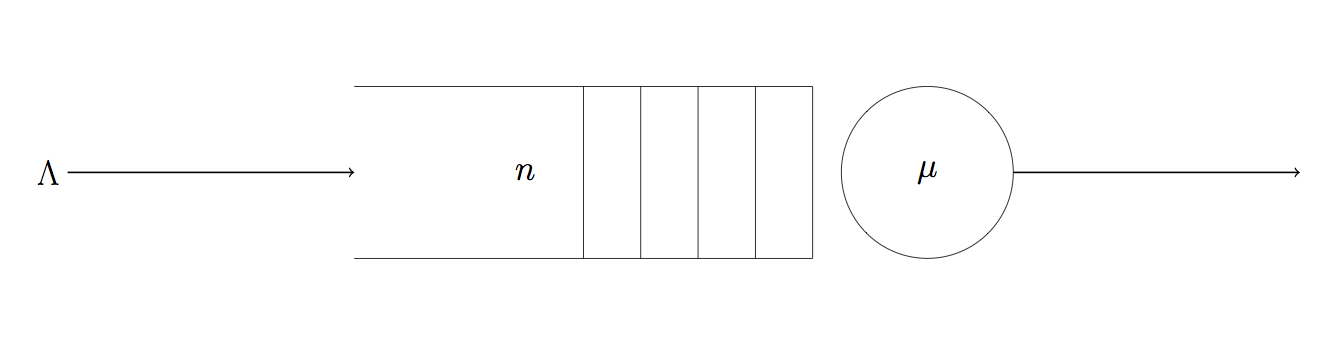
Challenge: Attempt to recreate this diagram of a queue using tikz:

6. Labels

Labels are how we can refer to earlier sections, figures, and equations (an many other things) in LaTeX. This is done through the \label{} command. To label a section, simply attach this command to the section command:

\section{Turtles}\label{sec:turtles}

Here, sec:turtles is the label I have given this section in order to easily refer to it. I can then call this section using \ref, for example:

Previously in Section~\ref{sec:turtles} turtles were discussed.

Notice the ~ here. This ensures that there will be no line break between the word ‘Section’ and the number yielded by the \ref command.

Figures and equations can also be labelled:

\begin{equation}\label{eqn:pythagoras}
a^2 + b^2 = c^2
\end{equation}

\begin{figure}
  \includegraphics[width=0.5\textwidth]{my_image.png}
  \caption{A brief description of the figure.}
  \label{fig:myimage}
\end{figure}

Challenge: In your article, label all sections, subsections, equations and figures. Write some sentences that refer to all these things.

7. Code

Including code snippets in your article can be done with another package called listings. First include the package in the preamble:

\usepackage{listings}

We can now include code in two ways, by directly typing in code, or by inputting a file. In order to type code in directly, use the lstlisting environment:

\begin{lstlisting}
for i in range(100):
    print(i ** 2)
\end{lstlisting}

If you already have code written in a file (for example a .py file, or a .R file), then you can use \lstinputlisting in a similar way to \includegraphics. You can even set the language of the code to ensure meaningful syntax highlighting (although you should check that your chosen language is supported):

\lstinputlisting[language=Python]{source_code.py}

Another great package for inluding code snippets is minted which allows for pretty syntax highlighting.

Challenge: Under your table of fruit, include a figure that shows the LaTeX code used to create that table. Include an appropriate caption, label the figure, and write some sentences that refer to in.

8. Environments

Everytime we began a section with a command starting with \begin{ and ended it with \end{, the content between those commands were in an environment. Here’a a list of some useful environments not covered so far:

• \begin{center} and \end{center}: Centers all the content.
• \begin{figure} and \end{figure}: An environment for figures, graphics, diagrams.
• \begin{table} and \end{table}: An environment similar to figure for tables with tabular.
• \begin{multicols} and \end{multicols}: An environment to set the text into columns.
• \begin{proof} and \end{proof}: An environment for writing mathematical proofs.

And using amsthm we get access to a number of commands for creating other useful environments. These are usually used for writing theorems, definitions, propositions, remarks and so on.

To define a new Theorem environment in the preable:

\usepackage{asmthm}

\newtheorem{theorem}{Theorem}

This gives us a numbered theorem environment that begins with the text Theorem. So we can write a theorem with proof as follows:

\begin{theorem}
  $\log_a{B} + \log_a{C} = \log_a{BC}$
\end{theorem}

\begin{proof}
  Let $x = \log_a{B}$ and $y = \log_a{C}$.
  Now:
  \begin{align}
    a^x a^y &= BC\\
    a^{x + y} &= BC\\
    x + y &= \log_a{BC}\\
    \log_a{B} + \log_a{C} &= \log_a{BC}
  \end{align}
  as required.
\end{proof}

Challenge: Choose two simple theorems and give their proofs by defining a new theorem environment.

Challenge: Create a definition environment and use it to define two mathematical terms.

9. Bibliographies

To produce bibliographies, references and citations, we need to include a .bib file containing the information of all the references we have used. This file should contain a list of entries that look similar to this:

@article{jackson57,
  author  = "Jackson, J.",
  title   = "Networks of waiting lines.",
  year    = "1957",
  journal = "Operations research",
  volume  = "5",
  number  = "4",
  pages   = "518--521"
}

The first line here jackson57 is the user-defined identifier, this is what you will use to refer to the article in your .tex file. All other lines describe the article itself. Obtaining this information is easy if using Google Scholar, simply search for the article, click Cite and then BibTeX.

You can cite many different types of information sources including books and websites, more information can be found here.

In order to refer to these in the main body, use the \cite command:

The study of queues routed into a network was first investigated in \cite{jackson57}.

Finally we must tell LaTeX where to look for the .bib file, and to output a bibliography. Let’s name our bib file refs.bib. At the end of your document (before \end{document}) insert:

\bibliographystyle{plain}
\bibliography{refs}

Challenge: Find an article, book, and (reputable) website, add then to a .bib file. Write some sentences that cite these sources, and add a bibliography to your article.

10. Presentations

So far we have only considered the article document class. Presentations like ‘powerpoint’ can be created using latex using the beamer document class. The preable of a beamer presentation will look like this:

\documentclass{beamer}

\begin{document}
% Your contents here...  
\end{document}

A presentation with Beamer consists of a series of ‘frames’. These contain content contained in a frame environment. A frame can have a title, set with \frametitle{:

\begin{frame}
  \frametitle{My frame's title}
  Content...
\end{frame}

Everything that has been discussed so far can be included in the frame’s conent: lists, tables, figures, mathematics and code. Beamer also has some further commands for manipulating overlays:

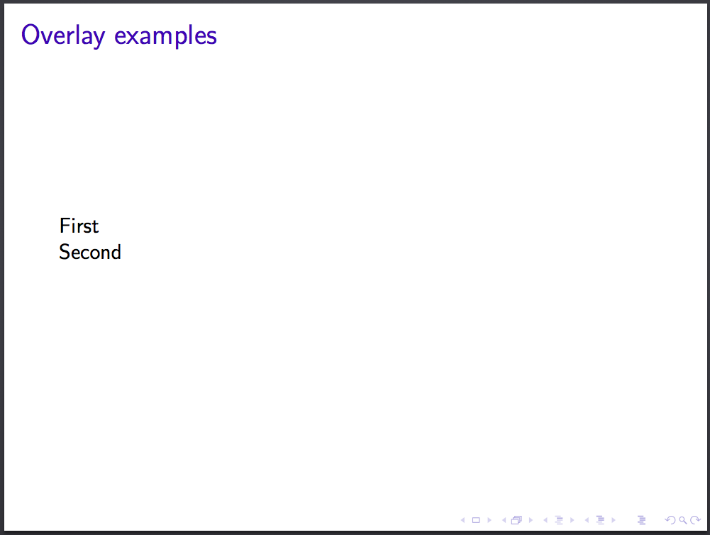
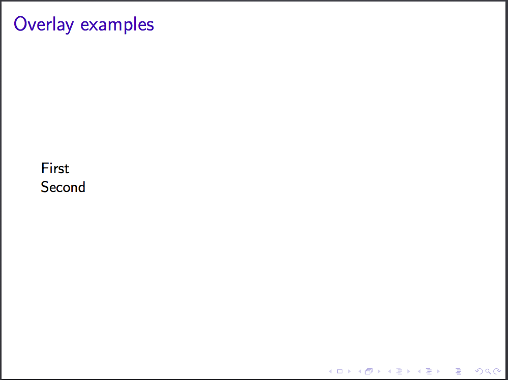
• \pause splits a frame: content before this command is put on one frame, and the next frame will contain the content both before and after this command.
• \onslide<3>{} and \only<3>{} are more flexible overlay options. The content within the curly brackets will only be displayed on the number overlay inside the < and > symbols; in this case only on the 3rd overlay. To display content on slides from the 3rd overlay onwards we can add a dash: <3->.

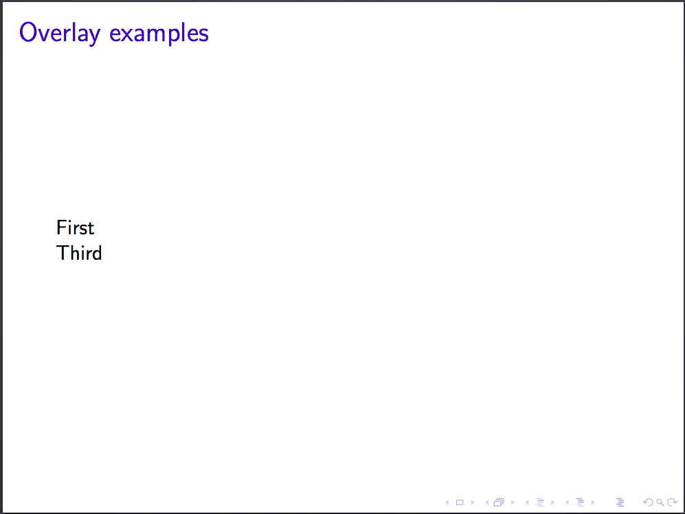
• Note that \onslide and \only have subtly different content positionings. Compare:

  \begin{frame}
    \frametitle{Overlay examples}
    \onslide<1->{First}
    
    \onslide<2>{Second}
    
    \onslide<3>{Third}
  \end{frame}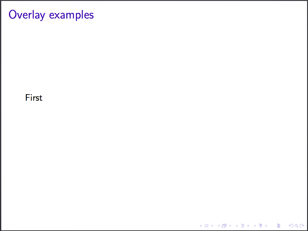
  

  

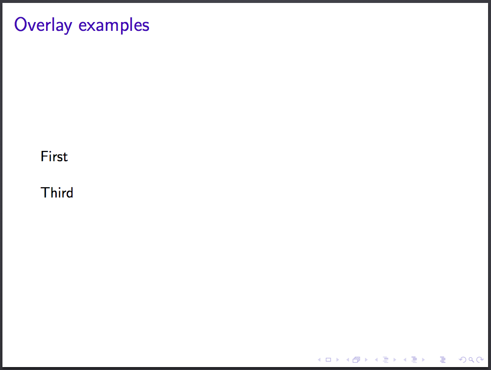
  to:

  \begin{frame}
    \frametitle{Overlay examples}
    \only<1->{First}
    
    \only<2>{Second}
    
    \only<3>{Third}
  \end{frame}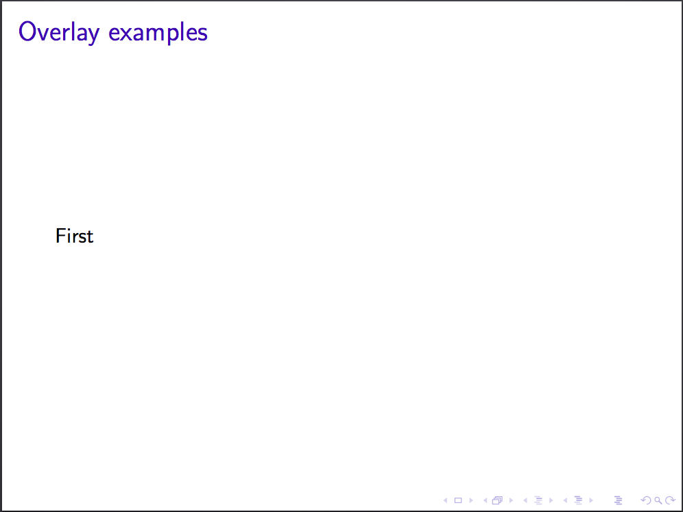
  

  

Beamer presentations can be customised with a theme and colour theme. To set these, use the following commands in the preable of your Beamer document (this example chooses the Singapore theme and crane colour theme):

\usetheme{Singapore}
\usecolortheme{crane}

Check out the beamer style matrix for examples of all combinations of themes and colour themes.

Challenge: Create a three frame presentation describing a mathematical theorem of your choice. Choose a theme and color theme, use mathematics, insert a figure, and experiment with overlay options.

Finally, many of you will find this template useful for writing your final year projects. Here’s a link to an Overleaf project with solutions to some of the challenges.