Inspection Bias in Queueing Systems
Why are buses always late? Why are my friends more popular than me? Inspection paradox. I recently recorded video lectures for my data literacy course next semester, and I briefly discuss the inspection paradox and inspection bias. It’s only a minor phenomenon, but is relevant to queueing systems, so understanding it might be interesting.
I think this blog post by Allen Downey explains it best - in the book Orange Is The New Black the author is sent to prison and is astonished that most of the people she meets are serving very long sentences, much longer than the average sentence length the judge issues. What’s going on? Inspection bias. Women serving shorter sentences spend less time in prison, so there’s less chance they’ll be there when you go to prison. Women serving longer sentences spend more time in prison, so there’s a higher chance they’ll be there when you go to prison.
Prisons are a queueing system with no buffer. So queueing systems must be prone to inspection bias. When parameterising a queueing model, if a full data set is unavailable, then we might take just “snapshots” of the system. For example if we want to know the sentence length distribution at a prison, we may enter the prison on some given days and ask the inmates there how long their sentence is. This collected data is subject to inspection bias, and so would need to be transformed back to it’s original distribution before using it to model the prison as a queueing system.
Consider two continuous random variables: \(X\) is the sentence length, with pdf \(f(x)\); and \(Y\) is the observed sentence length at these snapshots, with pdf \(g(x)\). What is the relationship between \(X\) and \(Y\)?
If Agatha has twice the sentence length of Barbara, then we’d expect the probability of observing Agatha in one of our snapshots to be twice the probability of observing Barbara. So it seems that the probability of observing a value is proportional to the value itself, as well as the true probability of that value occurring. So \(x f(x)\) is a good guess for \(g(x)\). To make sure this is a true pdf, we’d have to normalise this, so divide by \(\int x f(x)\), which just happens to be the expected value of \(X\). Therefore we can guess that:
\[g(x) = \frac{x f(x)}{\mathbb{E}[X]}\]Let’s check empirically with Ciw. Let’s say \(X \sim \text{Uniform}(3, 11)\), choose an arbitrary arrival distribution and infinite capacity:
>>> import ciw
>>> N = ciw.create_network(
...     arrival_distributions=[ciw.dists.Exponential(10)],
...     service_distributions=[ciw.dists.Uniform(3, 11)],
...     number_of_servers=[float('inf')]
... )
We’ll simulate this system initially for 500 time units to warm the system up, them take ‘snapshots’ at regular intervals and record the sentence lengths of the inmates present at those times:
>>> inspection_times = [500 + (i * 20) for i in range(100)]
>>> times = []
>>> for t in inspection_times:
...     Q.simulate_until_max_time(t)
...     times += [ind.service_time for ind in Q.nodes[1].all_individuals]
Now let’s compare the theoretical distributions \(f(x)\) and \(g(x)\), and the empirical distribution times obtained from the above code:
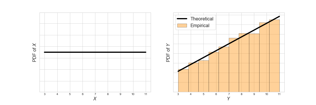
We see that inspection bias does indeed come into play here, and that our theoretical distribution \(g(x)\) fits the empirical distribution nicely. Let’s check again with a couple more different distributions.
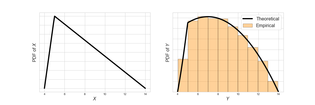
- A triangular distribution with positive skew, \(X \sim \text{Triangular}(4, 5, 14)\):
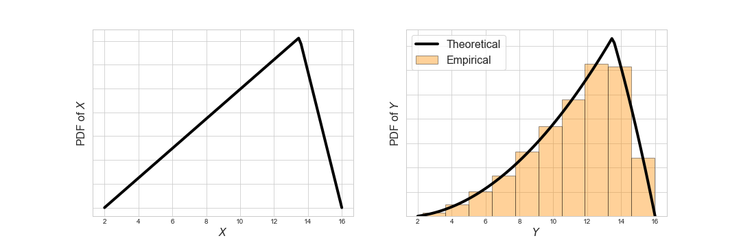
- A triangular distribution with negative skew, \(X \sim \text{Triangular}(2, 13.5, 16)\):
- An exponential distribution, \(X \sim \text{Expon}(2)\):
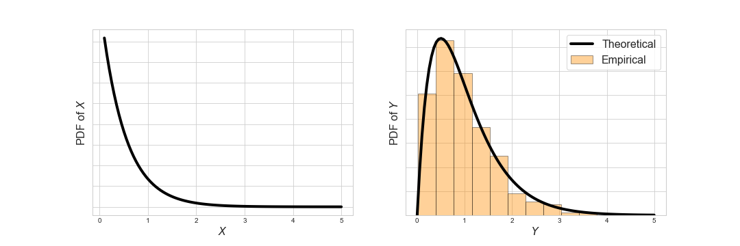
This is neat. It also works for queues with finite servers and a buffer, which just delays the observations (I don’t think it’ll work for prioritised queues however). Maybe our guess of the relationship between \(g(x)\) and \(f(x)\) is true. If so, given an empirical \(g(x)\) taken from snapshots of the system, we could transform it back to \(f(x)\) to use in our models:
\[f(x) = \frac{\mathbb{E}[X] g(x)}{x}\]Of course we do not know what \(\mathbb{E}[X]\) is yet, but that doesn’t matter, that’s only there to normalise is so that it’s a true pdf.
In Python:
>>> import matplotlib.pyplot as plt
>>> empirical = plt.hist(times)
>>> frequencies = empirical[0]
>>> midpoints = [(i + j) / 2 for i, j in zip(empirical[1][:-1], empirical[1][1:])]
>>> transformed = [p / x for x, p in zip(midpoints, frequencies)]![]()